Latent Variable Modelling in brms
I’ve been absent from this blog over the past few years. It seems I’ve been busy settling myself into my PhD! This is the first blog of 2020, and hopefully the first of many new statistical posts disseminating the various tidbits I’ve been learning during my PhD.
This blog post will cover modelling latent variables in the brms package in R. Latent variables are an important statistical concept in psychology, and I’ve found myself using them a lot in my PhD so far. But our options for statistically modelling latent variables, especially within Bayesian frameworks, are booming. Here’s a quick foray into this area.
What are latent variables?
Often, we are interested in studying variables which we cannot directly measure. For example, we may be interested in extraversion, a facet of personality that describes how outgoing and social someone is. There is no instrument or scientific measure that we can use to directly measure extraversion, at least not in the same way that we can directly measure distance in metres.
To get around this, psychologists often ask people batteries of validated questions, such as “I enjoy parties” and “I am outgoing and sociable”, that indirectly measure extraversion. Together, they assume that these questionnaire items predict a statistically unknown variable called a latent variable. This latent variable can simply be estimated, or can be used to predict other variables.
Using lavaan to measure latent variables
library(lavaan)
library(tidyverse)
The lavaan package in R is often used to measure latent variables. We will also use tidyverse to wrangle our data.
Let’s first create some simulated data to demonstrate this. We’ll create
an observed variable y that is normally distributed around 0 with a
standard deviation of 2.
y <- rnorm(n = 100, mean = 0, sd = 2)
Now we will create a latent variable x that is correlated with y. To make this
more concrete, imagine that x is extraversion, and y is something
that is predicted by extraversion, like ability to make people laugh at
parties.
x <- rnorm(n = 100, mean = y, sd = 2)
We simulated latent x and observed y to be positively correlated.
cor(x, y) %>% round(2)

## [1] 0.62
Unfortunately, since x is a latent variable, we can never know this
correlation for certain in the real world. Instead, we need to use
various measures of this latent variable, which we will call z1, z2,
and z3, to infer x. We add some noise around these manifest variables,
as none of them are perfect measures of x.
z1 <- rnorm(n = 100, mean = x, sd = 0.5)
z2 <- rnorm(n = 100, mean = x, sd = 0.5)
z3 <- rnorm(n = 100, mean = x, sd = 0.5)
Put these together into one dataframe.
d <- data.frame(y = y, x = x, z1 = z1, z2 = z2, z3 = z3)
rm(x, y, z1, z2, z3)
Now we will use lavaan to measure this latent variable.
fit <- cfa('X =~ z1 + z2 + z3', data = d)
summary(fit)

## lavaan 0.6-5 ended normally after 58 iterations
##
##   Estimator                                         ML
##   Optimization method                           NLMINB
##   Number of free parameters                          6
##
##   Number of observations                           100
##
## Model Test User Model:
##
##   Test statistic                                 0.000
##   Degrees of freedom                                 0
##
## Parameter Estimates:
##
##   Information                                 Expected
##   Information saturated (h1) model          Structured
##   Standard errors                             Standard
##
## Latent Variables:
##                    Estimate  Std.Err  z-value  P(>|z|)
##   X =~
##     z1                1.000
##     z2                0.987    0.032   31.284    0.000
##     z3                1.029    0.031   32.700    0.000
##
## Variances:
##                    Estimate  Std.Err  z-value  P(>|z|)
##    .z1                0.315    0.063    4.972    0.000
##    .z2                0.255    0.057    4.493    0.000
##    .z3                0.221    0.057    3.873    0.000
##     X                 5.844    0.871    6.710    0.000
How well have we estimated the latent variable?
d$x.pred <- predict(fit)
cor(d$x, d$x.pred) %>% as.numeric() %>% round(2)

## [1] 0.99
We estimated it pretty well. Can we also retrieve the correlation
between x and y?
fit <- cfa('X =~ z1 + z2 + z3; y ~ X', data = d)
standardizedSolution(fit)[4,4] %>% round(2)

## [1] 0.61
This is essentially the same as our correlation above. This is a trivial
example, because we actually know what x is in our data, but if we did
not, this latent variable approach would be the most valid way forward.
Here, just taking the mean of our continuous manifest variables gets us pretty close to the latent variable.
cor(d$x, apply(d[,c("z1","z2","z3")], 1, mean)) %>% round(2)

## [1] 0.99
But if we were using Likert scales, which we often do in psychology, taking the mean wouldn’t be valid.
Using brms
We can, however, take a Bayesian approach to this problem. The R package brms implements Bayesian regression. This package currently has latent variables in the works. But I thought I’d have a go here anyway.
In confirmatory factor analysis, we set one of the factor loadings to 1
as a constant. We cannot do this yet in brms, but we can set a stupidly
narrow prior such that no amount of data could feasibly shift it. Then
we use the missing data syntax mi() in brms to estimate the latent variable.
library(brms)

# add empty latent variable to data frame
d$X <- as.numeric(NA)

# mi(x) tells brms that it is missing
bf1 <- bf(z1 ~ 0 + mi(X)) # factor loading 1 (constant)
bf2 <- bf(z2 ~ 0 + mi(X)) # factor loading 2
bf3 <- bf(z3 ~ 0 + mi(X)) # factor loading 3
bf4 <- bf(X | mi() ~ 0)

fit2 <- brm(bf1 + bf2 + bf3 + bf4 + set_rescor(FALSE), data = d,
            prior = c(prior(normal(1, 0.000001), coef = miX, resp = z1),
                      prior(normal(1, 1), coef = miX, resp = z2),
                      prior(normal(1, 1), coef = miX, resp = z3)),
            iter = 4000, warmup = 2000, chains = 2, cores = 2,
            control = list(adapt_delta = 0.99, max_treedepth = 15))

save(fit2, file = "fit2.rda")
This takes a while to fit, but does eventually. Do we have similar parameters to those above?
summary(fit2)

##  Family: MV(gaussian, gaussian, gaussian, gaussian)
##   Links: mu = identity; sigma = identity
##          mu = identity; sigma = identity
##          mu = identity; sigma = identity
##          mu = identity; sigma = identity
## Formula: z1 ~ 0 + mi(X)
##          z2 ~ 0 + mi(X)
##          z3 ~ 0 + mi(X)
##          X | mi() ~ 0
##    Data: d (Number of observations: 100)
## Samples: 2 chains, each with iter = 4000; warmup = 2000; thin = 1;
##          total post-warmup samples = 4000
##
## Population-Level Effects:
##        Estimate Est.Error l-95% CI u-95% CI Rhat Bulk_ESS Tail_ESS
## z1_miX     1.00      0.00     1.00     1.00 1.00     3687     2299
## z2_miX     0.99      0.03     0.93     1.06 1.00     1073     1625
## z3_miX     1.03      0.03     0.97     1.10 1.00     1082     1654
##
## Family Specific Parameters:
##          Estimate Est.Error l-95% CI u-95% CI Rhat Bulk_ESS Tail_ESS
## sigma_z1     0.58      0.06     0.47     0.71 1.00     1530     1973
## sigma_z2     0.51      0.06     0.39     0.63 1.00     1126     1264
## sigma_z3     0.50      0.07     0.37     0.63 1.00      919     1331
## sigma_X      2.44      0.19     2.10     2.85 1.00     3949     2711
##
## Samples were drawn using sampling(NUTS). For each parameter, Eff.Sample
## is a crude measure of effective sample size, and Rhat is the potential
## scale reduction factor on split chains (at convergence, Rhat = 1).
Yes, loadings are the same. brms output gives us standard deviations instead of variances, which we can get by squaring.
brms also gives us posterior distributions for predicted factor scores. How similar are these to the ones lavaan gave us?
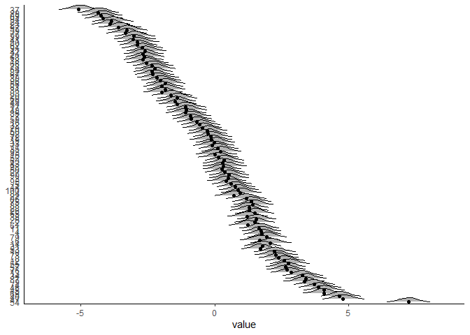
In the plot above, the dots are the predicted latent variable values from our lavaan model, and the distributions are the posterior densities for each individual’s Bayesian predicted factor score. They are very similar.
Finally, we can fit a structural equation model to see if this Bayesian
latent variable predicts y in the same way. We just add another formula
to the brm() call where y is predicted by the estimated latent variable
mi(x).
# add empty latent variable
d$X <- as.numeric(NA)

bf1 <- bf(z1 ~ 0 + mi(X)) # factor loading 1 (constant)
bf2 <- bf(z2 ~ 0 + mi(X)) # factor loading 2
bf3 <- bf(z3 ~ 0 + mi(X)) # factor loading 3
bf4 <- bf(X | mi() ~ 0)   # latent variable
bf5 <- bf(y ~ 0 + mi(X))  # added regression

fit3 <- brm(bf1 + bf2 + bf3 + bf4 + bf5 + set_rescor(FALSE), data = d,
            prior = c(prior(normal(1, 0.000001), coef = miX, resp = z1),
                      prior(normal(1, 1), coef = miX, resp = z2),
                      prior(normal(1, 1), coef = miX, resp = z3),
                      prior(normal(0, 1), coef = miX, resp = y)),
            iter = 4000, warmup = 2000, chains = 2, cores = 2,
            control = list(adapt_delta = 0.99, max_treedepth = 15))

save(fit3, file = "fit3.rda")
The unstandardised parameter for the relationship between latent x and
observed y in the lavaan model was:
parameterEstimates(fit)[4,4] %>% round(2)

## [1] 0.47
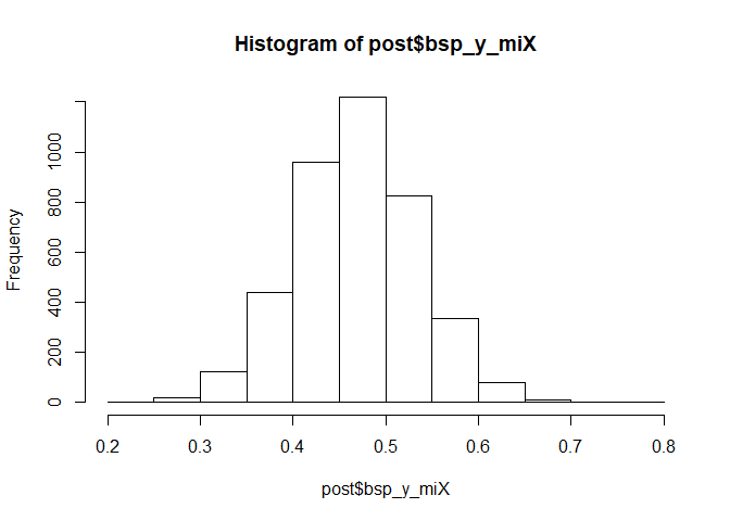
And in the brms model:
post <- posterior_samples(fit3)
median(post$bsp_y_miX) %>% round(2)

## [1] 0.47
Here’s the posterior distribution for that regression parameter. It’s
reliably above zero, suggesting a positive effect of latent x on
observed y.
hist(post$bsp_y_miX)
This shows that brms can handle confirmatory factor analysis and structural equation modelling with full Bayesian inference in Stan. Unfortunately, brms offers no good way of measuring model fit (except for comparing to other models), while lavaan offers a variety of model fit indices. For example:
fitMeasures(fit)['rmsea'] %>% round(2)

## rmsea
##  0.07

fitMeasures(fit)['srmr'] %>% round(2)

## srmr
## 0.01
These fit measures indicate good model fit. brms does offer the
pp_check() function though, which visualises model fit. For example,
let’s see how well the model predicts our outcome variable y.
pp_check(fit3, resp = "y", nsamples = 100)
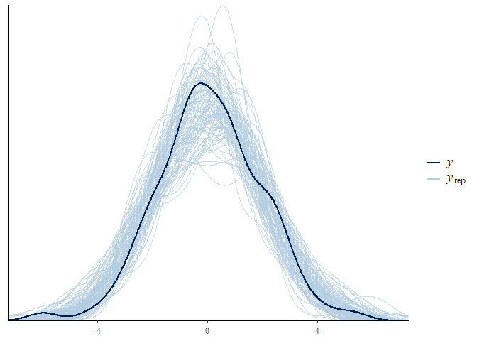
It does a pretty good job, though more data would make this a tighter fit.
The latent variable capabilities of brms are very exciting, and I look forward to their implementation in future versions of the package!
Session Info
sessionInfo()

## R version 3.6.1 (2019-07-05)
## Platform: x86_64-w64-mingw32/x64 (64-bit)
## Running under: Windows >= 8 x64 (build 9200)
##
## Matrix products: default
##
## locale:
## [1] LC_COLLATE=English_New Zealand.1252
## [2] LC_CTYPE=English_New Zealand.1252
## [3] LC_MONETARY=English_New Zealand.1252
## [4] LC_NUMERIC=C
## [5] LC_TIME=English_New Zealand.1252
##
## attached base packages:
## [1] stats     graphics  grDevices utils     datasets  methods   base
##
## other attached packages:
##  [1] ggridges_0.5.1  brms_2.10.0     Rcpp_1.0.2      lavaan_0.6-5
##  [5] forcats_0.4.0   stringr_1.4.0   dplyr_0.8.3     purrr_0.3.2
##  [9] readr_1.3.1     tidyr_1.0.0     tibble_2.1.3    ggplot2_3.2.1
## [13] tidyverse_1.2.1 rmarkdown_1.15
##
## loaded via a namespace (and not attached):
##  [1] nlme_3.1-140         matrixStats_0.55.0   xts_0.11-2
##  [4] lubridate_1.7.4      threejs_0.3.1        httr_1.4.1
##  [7] rstan_2.19.2         tools_3.6.1          backports_1.1.5
## [10] R6_2.4.0             DT_0.9               lazyeval_0.2.2
## [13] colorspace_1.4-1     withr_2.1.2          prettyunits_1.0.2
## [16] processx_3.4.1       tidyselect_0.2.5     gridExtra_2.3
## [19] mnormt_1.5-5         Brobdingnag_1.2-6    compiler_3.6.1
## [22] cli_1.1.0            rvest_0.3.4          shinyjs_1.0
## [25] xml2_1.2.2           labeling_0.3         colourpicker_1.0
## [28] scales_1.0.0         dygraphs_1.1.1.6     callr_3.3.2
## [31] StanHeaders_2.19.0   digest_0.6.21        pbivnorm_0.6.0
## [34] base64enc_0.1-3      pkgconfig_2.0.3      htmltools_0.3.6
## [37] htmlwidgets_1.3      rlang_0.4.0          readxl_1.3.1
## [40] rstudioapi_0.10      shiny_1.3.2          generics_0.0.2
## [43] zoo_1.8-6            jsonlite_1.6         crosstalk_1.0.0
## [46] gtools_3.8.1         inline_0.3.15        magrittr_1.5
## [49] loo_2.1.0            bayesplot_1.7.0      Matrix_1.2-17
## [52] munsell_0.5.0        abind_1.4-5          lifecycle_0.1.0
## [55] stringi_1.4.3        yaml_2.2.0           MASS_7.3-51.4
## [58] pkgbuild_1.0.5       plyr_1.8.4           grid_3.6.1
## [61] parallel_3.6.1       promises_1.0.1       crayon_1.3.4
## [64] miniUI_0.1.1.1       lattice_0.20-38      haven_2.1.1
## [67] hms_0.5.1            ps_1.3.0             zeallot_0.1.0
## [70] knitr_1.25           pillar_1.4.2         igraph_1.2.4.1
## [73] markdown_1.1         shinystan_2.5.0      codetools_0.2-16
## [76] reshape2_1.4.3       stats4_3.6.1         rstantools_2.0.0
## [79] glue_1.3.1           evaluate_0.14        modelr_0.1.5
## [82] vctrs_0.2.0          httpuv_1.5.2         cellranger_1.1.0
## [85] gtable_0.3.0         assertthat_0.2.1     xfun_0.9
## [88] mime_0.7             xtable_1.8-4         broom_0.5.2
## [91] coda_0.19-3          later_0.8.0          rsconnect_0.8.15
## [94] shinythemes_1.1.2    ellipsis_0.3.0       bridgesampling_0.7-2