Analysing Data on Contagious Yawning
Recently, we published a paper in Proceedings of the Royal Society B on contagious yawning in dogs. The paper argued against the idea that contagious yawning is a valid measure of empathy, showing that several predictions of the contagious-yawning-empathy hypothesis were not met in a re-analysis of previous studies of dogs and a novel experiment.
As my first scientific publication, I’m very proud of this paper. However, I’m not going to go into much detail about the arguments in the paper. Instead, I want to focus on the statistical analyses. We came across some challenges when analysing these data, and I’d like to get our approach down on paper so that someone with the same kind of dataset might be helped somewhere down the line.
First, let’s have a look at the data in question.
# you can find these data at https://osf.io/qru5s/
d <- read.csv("yawnReanalysis.csv")
head(d)

##   ID    study numberYawns age gender trial condition presentation type demonstrator   familiar live secs
## 1 P1 JM et al           1   5      M     2   Yawning          V+A  Pet        Human Unfamiliar Live  300
## 2 P2 JM et al           5   8      M     2   Yawning          V+A  Pet        Human Unfamiliar Live  300
## 3 P3 JM et al           1   7      M     1   Yawning          V+A  Pet        Human Unfamiliar Live  300
## 4 P4 JM et al           1   4      F     2   Yawning          V+A  Pet        Human Unfamiliar Live  300
## 5 P5 JM et al           2   5      F     1   Yawning          V+A  Pet        Human Unfamiliar Live  300
## 6 P6 JM et al           0  15      M     2   Yawning          V+A  Pet        Human Unfamiliar Live  300
This dataset combines the data from six previous studies of contagious
yawning in dogs. Each study used the following methodology: observe the
dog for a particular observation window (secs) and count the number of
yawns (numberYawns). There are two different experimental conditions
(condition) in these studies: (1) a Control condition where a
demonstrator is not yawning, and (2) a Yawning condition where a
demonstrator is yawning.
Before going any further, let’s have a closer look at the distribution
of the dependent variable numberYawns.
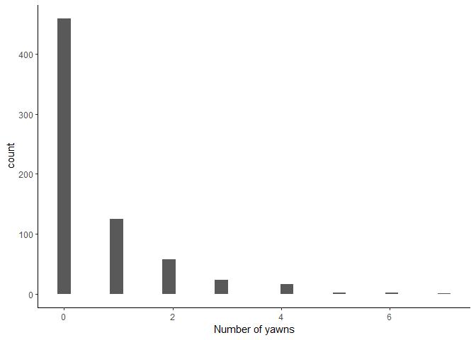
Since this is a count variable, we know up-front that we should probably
model these data with a Poisson distribution. But we can see lots of
zeroes in these data too - later, we’ll try and deal with these. But for
now, let’s just fit a simple intercept-only Poisson model. We use the
package brms for all our modelling.
library(brms)

# intercept-only Poisson model
m1 <- brm(numberYawns ~ 1, data = d, family = poisson)
m1 <- add_criterion(m1, "loo")
save(m1, file = "m1.rda")
How well did this model fit the data?
pp_check(m1)
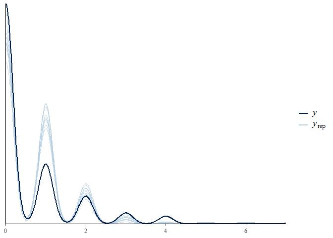
This model is okay. It’s predicting integer data, which is correct in this case, though it seems to be underestimating the number of zeroes and overestimating the number of ones. This is likely because, as we’ve already established, these data are severely zero-inflated.
Before tackling that, though, we should first acknowledge a fundamental flaw in the model we have already fitted. It does not take into account different exposure lengths in different studies.
unique(d$secs)

## [1] 300  50 180 600
Some studies observed the dogs for 50 seconds, some studies observed them for 10 minutes. This is very important - some studies may have simply observed more yawns because they measured for longer. To deal with this, we include an “offset” in our model. This basically turns the left hand side of the equation into a “rate per second”.
# intercept-only Poisson model with offset
m2 <- brm(numberYawns ~ 1 + offset(log(secs)), data = d, family = poisson)
m2 <- add_criterion(m2, "loo")
save(m2, file = "m2.rda")
Does this model fit a little better?
pp_check(m2)
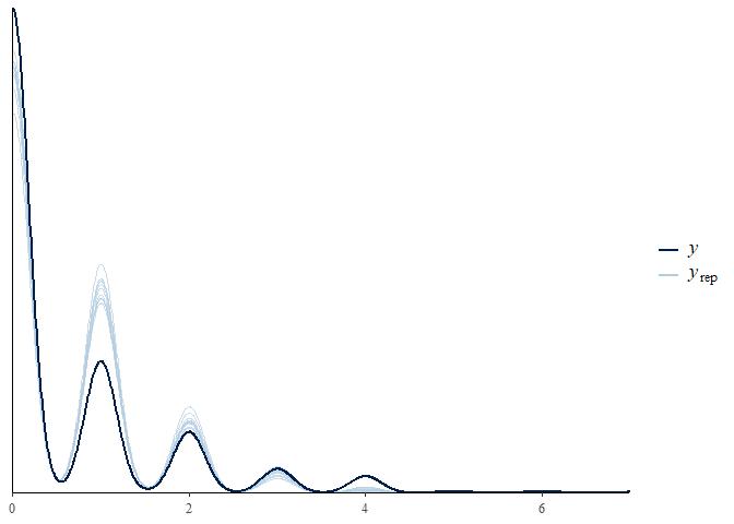
It still seems to be underestimating zeroes and overestimating ones.
loo_compare(m1, m2)

##    elpd_diff se_diff
## m2   0.0       0.0
## m1 -61.1      16.2
Nevertheless, leave-one-out cross-validation suggests that including the offset does improve model fit.
Let’s now try and improve model fit even more by accounting for zero-inflation. The class of model we settled on in the paper is a hurdle Poisson model. This is a mixture model that simultaneously models two separate processes. The first process is a Bernoulli process that determines whether the dependent variable is zero or a positive count. The second process is a Poisson process that determines the count once we know the dependent variable is positive (i.e. the model has “got over” the first hurdle).
# intercept-only hurdle Poisson model with offset
m3 <- brm(bf(numberYawns ~ 1 + offset(log(secs)), # Poisson process
             hu ~ 1),                             # Bernoulli process
          data = d, family = hurdle_poisson)
m3 <- add_criterion(m3, "loo")
save(m3, file = "m3.rda")

pp_check(m3)
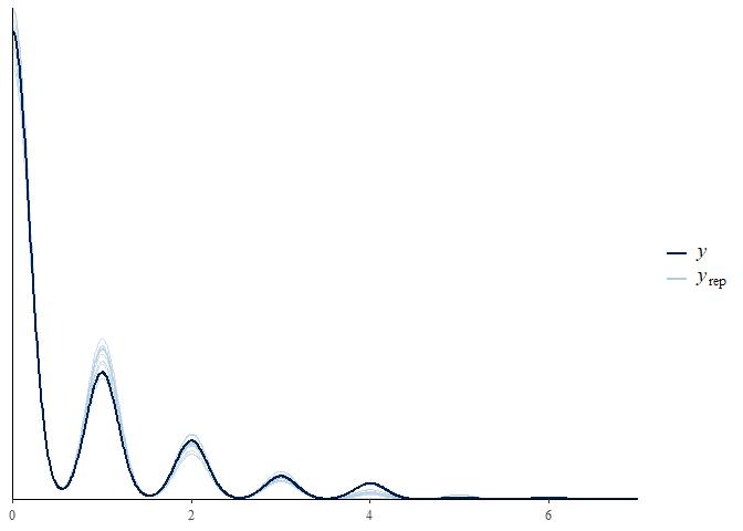
This model seems to be doing better with the zeroes and ones. Has it improved the fit?
loo_compare(m2, m3)

##    elpd_diff se_diff
## m3  0.0       0.0
## m2 -1.2      15.0
Interestingly, it has, but not by a huge amount.
What’s the probability of zeroes predicted by this model?
post <- posterior_samples(m3)
median(inv_logit_scaled(post$b_hu_Intercept)) %>% round(2)

## [1] 0.67
And the rate of yawning per minute?
(exp(post$b_Intercept) * 60) %>% median() %>% round(2)

## [1] 0.17
There’s one other aspect of the data that we haven’t taken into account.
Model m3 does not acknowledge that observations are nested within
individuals, and individuals are nested within studies. We can account
for this non-independence by including random intercepts for individuals
within studies (1|study/ID), for both parts of the model.
# intercept-only hurdle Poisson model with offset and random intercepts
m4 <- brm(bf(numberYawns ~ 1 + offset(log(secs)) + (1|study/ID),
             hu ~ 1 + (1|study/ID)),
          data = d, family = hurdle_poisson,
          control = list(adapt_delta = 0.9))
m4 <- add_criterion(m4, "loo")
save(m4, file = "m4.rda")

pp_check(m4) +
  scale_x_continuous(limits = c(0, 7))
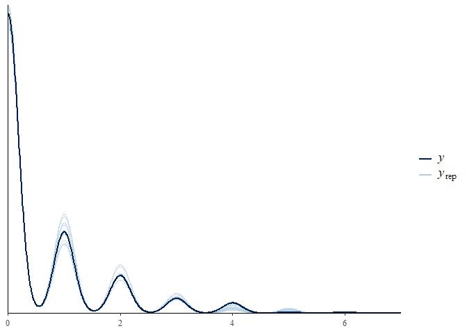
This is the best fit we’ve seen yet. Does a final model comparison confirm this?
loo_compare(m1, m2, m3, m4)

##    elpd_diff se_diff
## m4    0.0       0.0
## m3  -56.7      11.1
## m2  -57.8      13.2
## m1 -119.0      18.9
m4 knocks it out of the park. Clearly there are important
individual-level and study-level differences that this model accounts
for. Let’s visualise the study-level posterior differences.
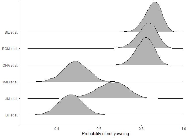
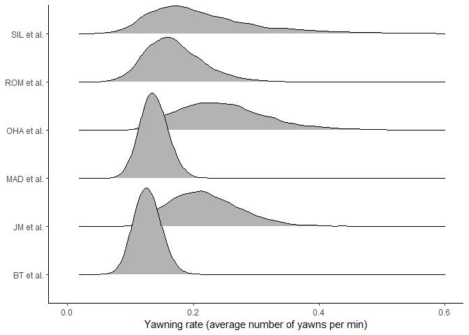
There are clearly large differences between studies in both the probability of yawning at all (the Bernoulli process) and the rate of yawning (the Poisson process). For example, SIL et al. has a high probability of zeroes and large uncertainty in yawning rate, whereas BT et al. has a low probability of zeroes and more certainty in the yawning rate. These differences are important to account for in the model.
And so, with incremental steps, we have created a model skeleton that we
think is describing the data generating process well. But we haven’t
even added any predictors yet! I will leave it up to the interested
reader to add condition as a predictor. You can do this for both
processes in the hurdle model (i.e. predicting the probability of zeroes
and the rate of yawning separately). Or if you want to just find out the
results of this kind of analysis, you can check out our
paper.
Hopefully, this blog post will encourage people to use their expertise and prior knowledge about the data to find a model that is suited to them. Rather than blindly throwing everything into an ANOVA and seeing what works!
sessionInfo()

## R version 3.6.2 (2019-12-12)
## Platform: x86_64-w64-mingw32/x64 (64-bit)
## Running under: Windows >= 8 x64 (build 9200)
##
## Matrix products: default
##
## locale:
## [1] LC_COLLATE=English_New Zealand.1252  LC_CTYPE=English_New Zealand.1252    LC_MONETARY=English_New Zealand.1252 LC_NUMERIC=C                         LC_TIME=English_New Zealand.1252
##
## attached base packages:
## [1] stats     graphics  grDevices utils     datasets  methods   base
##
## other attached packages:
##  [1] ggridges_0.5.2  brms_2.11.6     Rcpp_1.0.3      forcats_0.4.0   stringr_1.4.0   dplyr_0.8.4     purrr_0.3.3     readr_1.3.1     tidyr_1.0.2     tibble_2.1.3    ggplot2_3.2.1   tidyverse_1.3.0 rmarkdown_2.1   knitr_1.28
##
## loaded via a namespace (and not attached):
##  [1] nlme_3.1-144         matrixStats_0.55.0   fs_1.3.1             xts_0.12-0           lubridate_1.7.4      threejs_0.3.3        httr_1.4.1           rstan_2.19.2         tools_3.6.2          backports_1.1.5      R6_2.4.1             DT_0.12              DBI_1.1.0            lazyeval_0.2.2       colorspace_1.4-1     withr_2.1.2          prettyunits_1.1.1    processx_3.4.2       gridExtra_2.3        tidyselect_1.0.0     Brobdingnag_1.2-6    compiler_3.6.2       cli_2.0.1
## [24] rvest_0.3.5          shinyjs_1.1          xml2_1.2.2           labeling_0.3         colourpicker_1.0     scales_1.1.0         dygraphs_1.1.1.6     mvtnorm_1.0-11       callr_3.4.2          StanHeaders_2.21.0-1 digest_0.6.23        base64enc_0.1-3      pkgconfig_2.0.3      htmltools_0.4.0      dbplyr_1.4.2         fastmap_1.0.1        htmlwidgets_1.5.1    rlang_0.4.4          readxl_1.3.1         rstudioapi_0.11      shiny_1.4.0          farver_2.0.3         generics_0.0.2
## [47] zoo_1.8-7            jsonlite_1.6.1       gtools_3.8.1         crosstalk_1.0.0      inline_0.3.15        magrittr_1.5         loo_2.2.0            bayesplot_1.7.1      Matrix_1.2-18        munsell_0.5.0        fansi_0.4.1          abind_1.4-5          lifecycle_0.1.0      stringi_1.4.4        yaml_2.2.1           pkgbuild_1.0.6       plyr_1.8.5           grid_3.6.2           parallel_3.6.2       promises_1.1.0       crayon_1.3.4         miniUI_0.1.1.1       lattice_0.20-38
## [70] haven_2.2.0          hms_0.5.3            ps_1.3.0             pillar_1.4.3         igraph_1.2.4.2       markdown_1.1         shinystan_2.5.0      stats4_3.6.2         reshape2_1.4.3       rstantools_2.0.0     reprex_0.3.0         glue_1.3.1           evaluate_0.14        modelr_0.1.5         vctrs_0.2.2          httpuv_1.5.2         cellranger_1.1.0     gtable_0.3.0         assertthat_0.2.1     xfun_0.12            mime_0.9             xtable_1.8-4         broom_0.5.4
## [93] coda_0.19-3          later_1.0.0          rsconnect_0.8.16     shinythemes_1.1.2    ellipsis_0.3.0       bridgesampling_0.8-1