I recently posted a pre-print on PsyArxiv entitled “The non-independence of nations and why it matters”. In the paper, myself and Quentin Atkinson argue that many cross-national correlations in the social sciences are flawed because they do not adequately take into account various forms of non-independence between nations. Nations are linked to one another via spatial proximity and shared cultural ancestry, and failing to account for these dependencies can increase the chance of false positives.

That’s the issue: but how to rectify it? In the paper, we suggest some Bayesian modelling techniques that researchers can use to overcome the problem. However, we did not go into these techniques in detail. So I thought it would be useful to provide a brief R tutorial on the methods we used in the paper, so that interested researchers can apply them to their own cross-national datasets.

In this blog post, I will walk through methods of dealing with (1) spatial non-independence, and (2) cultural phylogenetic non-independence. In each case, I will use simulated data, show that a naive cross-national correlation produces an inflated effect size, and then present an alternative method that controls for non-independence. The techniques I will use are not the only ways of dealing with non-independence, but they are the techniques I learned through folks like Richard McElreath and Paul-Christian Bürkner.

For this tutorial, we will need the following R packages: tidyverse for plotting and data wrangling, brms for fitting Bayesian models, ggcorrplot for plotting proximity matrices, ggrepel for neatly plotting country labels, readxl for reading in Excel files, and targets for extracting objects from our reproducible analysis pipeline.

library(tidyverse)
library(brms)
library(ggcorrplot)
library(ggrepel)
library(readxl)
library(targets)

The data and code for this vignette can be found on GitHub: https://github.com/ScottClaessens/crossNationalCorrelations

Spatial non-independence

Spatially non-independent simulated data

For this demonstration, we load a subset of OECD nations from one of the many simulated datasets from our paper. This dataset contains a standardised predictor variable (X) and a standardised outcome variable (Y), both of which are strongly spatially autocorrelated.

# load dataset from file
spatialSimData <- read.csv("data/vignette/spatialSimData.csv")

We can plot the relationship between the nation-level predictor and outcome variables.

ggplot(spatialSimData, aes(x, y, label = country)) +
  geom_point() +
  geom_text_repel() +
  geom_smooth(method = "lm") +
  theme_classic()

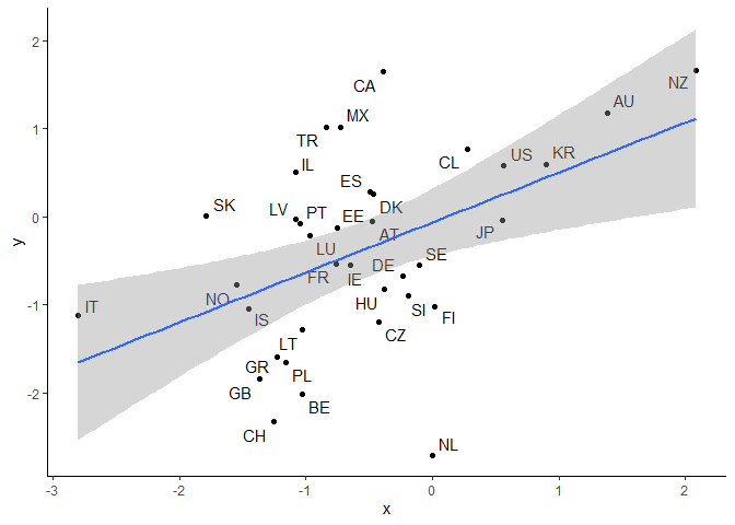
The relationship between the simulated variables appears to be positive. But is this just due to spatial non-independence? From the plot, it looks like this might be the case. For example, neighbouring countries, such as Sweden (SE) and Finland (FI), have very similar values on both variables, while the distant countries Australia (AU) and New Zealand (NZ) are far off in the top right hand corner of the plot.

Fit naive correlation

We can easily get the naive Pearson’s correlation between the national-level variables.

cor(spatialSimData$y, spatialSimData$x) %>% round(2)

## [1] 0.48

We can also get this same correlation from fitting a Bayesian regression. This is where we use the R package brms. We set some regularising priors on the intercept, slope, and residual variance in this model.

# fit naive bayesian regression
m1.1 <- brm(y ~ x, data = spatialSimData, 
            cores = 4, seed = 2113,
            # regularising priors
            prior = c(prior(normal(0, 1), class = Intercept),
                      prior(normal(0, 1), class = b),
                      prior(exponential(2), class = sigma)))

# get model summary
summary(m1.1)

##  Family: gaussian 
##   Links: mu = identity; sigma = identity 
## Formula: y ~ x 
##    Data: spatialSimData (Number of observations: 36) 
##   Draws: 4 chains, each with iter = 2000; warmup = 1000; thin = 1;
##          total post-warmup draws = 4000
## 
## Population-Level Effects: 
##           Estimate Est.Error l-95% CI u-95% CI Rhat Bulk_ESS Tail_ESS
## Intercept    -0.06      0.19    -0.44     0.32 1.00     3205     2621
## x             0.55      0.17     0.21     0.87 1.00     3513     2908
## 
## Family Specific Parameters: 
##       Estimate Est.Error l-95% CI u-95% CI Rhat Bulk_ESS Tail_ESS
## sigma     0.97      0.12     0.78     1.23 1.00     3012     2261
## 
## Draws were sampled using sampling(NUTS). For each parameter, Bulk_ESS
## and Tail_ESS are effective sample size measures, and Rhat is the potential
## scale reduction factor on split chains (at convergence, Rhat = 1).

Because both variables are standardised, the slope is comparable to the Pearson’s correlation reported above. The model converged normally, and the 95% credible interval for the slope is above zero. In other words, this is a “significantly positive” relationship.

Fit correlation with Gaussian Process

But is spatial non-independence ruining our inference? To find out, we fit another model including a Gaussian Process over latitudes and longitudes for nations. A Gaussian Process adds a random intercept for each nation, and these random intercepts are allowed to covary according to the distance between latitude-longitude coordinates. For a more detailed discussion of this method of dealing with spatial autocorrelation, see Section 14.5 in Richard McElreath’s book Statistical Rethinking (second edition), or his 2022 lecture on the topic here.

We can include Gaussian Processes in brms models using the gp() function. This function takes a variable — or multiple variables, in our case — and, under the hood, computes a normalised distance matrix between all the cases for that variable. It then estimates a covariance function specifying how these distances relate to the covariance between nations. If the data are spatially autocorrelated, the model will estimate strong spatial covariance between nations, which could “soak up” much of the relationship we saw in the previous section.

We fit this model by adding a gp() term to our formula.

# fit Bayesian regression with Gaussian Process
m1.2 <- brm(y ~ x + gp(latitude, longitude), 
            data = spatialSimData, cores = 4, seed = 2113,
            # regularising priors
            prior = c(prior(normal(0, 1), class = Intercept),
                      prior(normal(0, 1), class = b),
                      prior(exponential(2), class = sdgp),
                      prior(exponential(2), class = sigma)),
            # tune the mcmc sampler
            control = list(adapt_delta = 0.99))

# get model summary
summary(m1.2)

##  Family: gaussian 
##   Links: mu = identity; sigma = identity 
## Formula: y ~ x + gp(latitude, longitude) 
##    Data: spatialSimData (Number of observations: 36) 
##   Draws: 4 chains, each with iter = 2000; warmup = 1000; thin = 1;
##          total post-warmup draws = 4000
## 
## Gaussian Process Terms: 
##                             Estimate Est.Error l-95% CI u-95% CI Rhat Bulk_ESS Tail_ESS
## sdgp(gplatitudelongitude)       0.59      0.28     0.09     1.22 1.00     1294      857
## lscale(gplatitudelongitude)     0.09      0.08     0.02     0.28 1.00     1474     1975
## 
## Population-Level Effects: 
##           Estimate Est.Error l-95% CI u-95% CI Rhat Bulk_ESS Tail_ESS
## Intercept     0.30      0.35    -0.32     1.03 1.00     2103     2585
## x             0.32      0.22    -0.13     0.74 1.00     2853     2917
## 
## Family Specific Parameters: 
##       Estimate Est.Error l-95% CI u-95% CI Rhat Bulk_ESS Tail_ESS
## sigma     0.83      0.12     0.63     1.09 1.00     2289     2854
## 
## Draws were sampled using sampling(NUTS). For each parameter, Bulk_ESS
## and Tail_ESS are effective sample size measures, and Rhat is the potential
## scale reduction factor on split chains (at convergence, Rhat = 1).

As expected, the slope has reduced in size, and the 95% credible interval now includes zero. This suggests that the positive relationship we initially found in our naive regression was confounded by spatial non-independence.

Cultural phylogenetic non-independence

Culturally non-independent simulated data

It is also possible for nations to be culturally non-independent — that is, they share common influences from shared cultural ancestors. For example, even though the United Kingdom and New Zealand are on opposite sides of the planet, they are culturally similar due to the effects of British colonialism. This source of non-independence can be just as important as spatial proximity, especially when we are interested in cultural norms and institutions.

As before, we load a subset of OECD nations from a simulated dataset containing a standardised predictor variable (X) and a standardised outcome variable (Y). Both of these variables are strongly culturally autocorrelated.

# load dataset from file
culturalSimData <- read.csv("data/vignette/culturalSimData.csv")

Let’s plot the relationship between the nation-level predictor and outcome variables.

ggplot(culturalSimData, aes(x, y, label = country)) +
  geom_point() +
  geom_text_repel() +
  geom_smooth(method = "lm") +
  theme_classic()

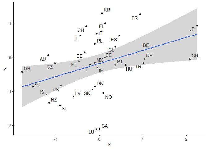
There’s a positive relationship between the variables. But a close look at the plot suggests some cultural clustering. For example, the English-speaking nations Australia (AU), New Zealand (NZ), the United States (US), and the United Kingdom (GB) are all towards the left of the plot, whereas nations speaking more distantly related languages, such as Japan (JP) and Greece (GR), are further to the right.

Fit naive correlation

As before, we can get the naive Pearson’s correlation.

cor(culturalSimData$y, culturalSimData$x) %>% round(2)

## [1] 0.4

And we can estimate this correlation in a naive Bayesian regression model.

# fit naive bayesian regression
m2.1 <- brm(y ~ x, data = culturalSimData, 
            cores = 4, seed = 2113,
            # regularising priors
            prior = c(prior(normal(0, 1), class = Intercept),
                      prior(normal(0, 1), class = b),
                      prior(exponential(2), class = sigma)))

# get model summary
summary(m2.1)

##  Family: gaussian 
##   Links: mu = identity; sigma = identity 
## Formula: y ~ x 
##    Data: culturalSimData (Number of observations: 36) 
##   Draws: 4 chains, each with iter = 2000; warmup = 1000; thin = 1;
##          total post-warmup draws = 4000
## 
## Population-Level Effects: 
##           Estimate Est.Error l-95% CI u-95% CI Rhat Bulk_ESS Tail_ESS
## Intercept    -0.18      0.13    -0.44     0.08 1.00     3538     2960
## x             0.38      0.15     0.09     0.68 1.00     3554     2725
## 
## Family Specific Parameters: 
##       Estimate Est.Error l-95% CI u-95% CI Rhat Bulk_ESS Tail_ESS
## sigma     0.81      0.10     0.64     1.03 1.00     3688     2931
## 
## Draws were sampled using sampling(NUTS). For each parameter, Bulk_ESS
## and Tail_ESS are effective sample size measures, and Rhat is the potential
## scale reduction factor on split chains (at convergence, Rhat = 1).

The 95% credible interval for the slope is above zero, suggesting that there is a “significantly positive” relationship.

Fit correlation with covarying random effects

“Cultural similarity” does not have a fixed coordinate system like longitude and latitude, making Gaussian Processes tricky in brms. Instead, we can use another technique that allows nation random intercepts to covary, but we specify the covariance matrix in advance rather than estimate it in the model. This will allow us to control for cultural non-independence.

What covariance matrix should we specify in advance? The matrix that we use in the paper is the linguistic proximity between nations, weighted by the proportion of speakers of each language in each nation. “Linguistic proximity” here means how related two languages are on a phylogeny of languages. We just average this measure over all languages spoken in each nation, weighted by speaker percentages. This gives us a sense of how “culturally similar” different nations are.

It is simpler to just show the matrix. Below, we load the full linguistic distance matrix, subset it to just our OECD nations, and convert it to a linguistic proximity matrix.

# load full linguistic distance matrix
linDist <- 
  read_xlsx("data/networks/2F Country Distance 1pml adj.xlsx") %>%
  select(-ISO) %>%
  as.matrix()

# rows and columns identical in symmetrical matrix
rownames(linDist) <- colnames(linDist)

# subset to only OECD countries
linDist <- linDist[oecd,oecd]

# nation's distance from itself is zero
diag(linDist) <- 0

# normalise between 0 and 1
linDist <- linDist / max(linDist)

# convert to linguistic proximity
linProx <- 1 - linDist

We can then plot this linProx object, to get a sense of the cultural relatedness of different nations.

ggcorrplot(linProx, hc.order = TRUE, type = "lower") +
  theme(legend.title = element_blank())

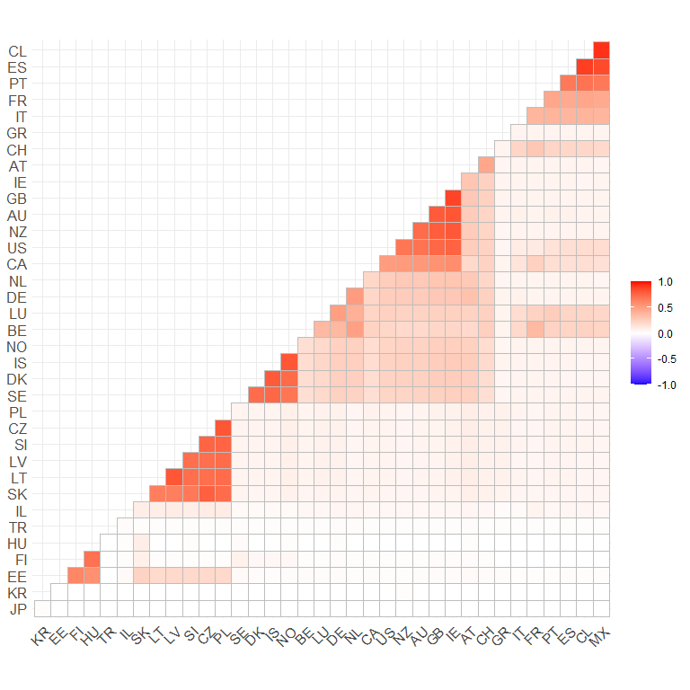
From this plot, we can see that majority English-speaking nations have high linguistic proximity (i.e. cultural similarity), as do Scandinavian nations, nations in Western Europe, and nations in Eastern Europe.

We can use this linguistic proximity matrix in our modelling. In brms, we can specify in advance how our random effects should be correlated by using the cov argument in the gr() function. The only restrictions are that the matrix that we feed in must have row and column names that match our variable, and that the matrix is positive definite. To learn more about this method, see this vignette on phylogenetic regression from Paul-Christian Bürkner.

# fit bayesian regression with covarying random effects
m2.2 <- brm(y ~ x + (1 | gr(country, cov = linProx)), 
            data = culturalSimData, cores = 4, seed = 2113,
            # pre-specified covariance matrix must be passed to brms via data2 argument
            data2 = list(linProx = linProx),
            # regularising priors
            prior = c(prior(normal(0, 1), class = Intercept),
                      prior(normal(0, 1), class = b),
                      prior(exponential(2), class = sd),
                      prior(exponential(2), class = sigma)),
            # tune mcmc sampler
            control = list(adapt_delta = 0.999))

# get model summary
summary(m2.2)

## Warning: There were 5 divergent transitions after warmup. Increasing adapt_delta above 0.999 may help. See http://mc-stan.org/misc/warnings.html#divergent-transitions-after-warmup

##  Family: gaussian 
##   Links: mu = identity; sigma = identity 
## Formula: y ~ x + (1 | gr(country, cov = linProx)) 
##    Data: culturalSimData (Number of observations: 36) 
##   Draws: 4 chains, each with iter = 2000; warmup = 1000; thin = 1;
##          total post-warmup draws = 4000
## 
## Group-Level Effects: 
## ~country (Number of levels: 36) 
##               Estimate Est.Error l-95% CI u-95% CI Rhat Bulk_ESS Tail_ESS
## sd(Intercept)     0.62      0.36     0.03     1.23 1.02       77      330
## 
## Population-Level Effects: 
##           Estimate Est.Error l-95% CI u-95% CI Rhat Bulk_ESS Tail_ESS
## Intercept    -0.03      0.27    -0.50     0.57 1.01      820      878
## x             0.30      0.17    -0.04     0.63 1.00     1500     1527
## 
## Family Specific Parameters: 
##       Estimate Est.Error l-95% CI u-95% CI Rhat Bulk_ESS Tail_ESS
## sigma     0.55      0.25     0.07     0.93 1.03       59       79
## 
## Draws were sampled using sampling(NUTS). For each parameter, Bulk_ESS
## and Tail_ESS are effective sample size measures, and Rhat is the potential
## scale reduction factor on split chains (at convergence, Rhat = 1).

Note that there were a number of divergent transitions, even after we increased adapt_delta, and the number of effective samples are not great. But the Rhat values are all beneath 1.05, suggesting that this model is reasonable.

As expected, we find that the positive relationship between our variables goes away when we control for cultural phylogenetic non-independence between nations.

Applying these methods in your research

There are a number of advantages to using Gaussian Processes and covarying random effects to deal with various forms of non-independence, beyond what I’ve outlined here. Both methods are possible to use when we have multiple data points per nation. Both methods can also be used for any conceivable likelihood — logistic regression for binary variables, cumulative link regression for ordinal variables, beta regression for variables bounded between 0 and 1, etc. All of this is possible using the brms package.

Happy cross-national modelling!