Ancestral state reconstruction
Erik Ringen
2026-10-06
Source:vignettes/ancestral_states.Rmd
ancestral_states.RmdOverview
The coev_ancestral_states() function extracts posterior
estimates of latent trait values at internal (ancestral) nodes of the
phylogeny from a fitted coevfit model. Because the model
estimates latent states at every node in the tree, ancestral state
reconstruction is a natural byproduct of model fitting – no separate
analysis is needed.
This vignette demonstrates the function using the authority dataset bundled with the package: political and religious authority among 97 Austronesian societies.
Fit the model
We fit a coevolutionary model with two ordered-logistic variables. For demonstration purposes we use moderate sampling settings; in practice you would want more iterations and to check convergence carefully.
fit <- coev_fit(
  data = authority$data,
  variables = list(
    political_authority = "ordered_logistic",
    religious_authority = "ordered_logistic"
  ),
  id = "language",
  tree = authority$phylogeny,
  parallel_chains = 4,
  chains = 4,
  iter_sampling = 500,
  iter_warmup = 500,
  seed = 42
)
Running MCMC with 4 parallel chains...
Chain 1 Iteration: 1 / 1000 [ 0%] (Warmup)
Chain 2 Iteration: 1 / 1000 [ 0%] (Warmup)
Chain 3 Iteration: 1 / 1000 [ 0%] (Warmup)
Chain 4 Iteration: 1 / 1000 [ 0%] (Warmup)
Chain 1 Iteration: 100 / 1000 [ 10%] (Warmup)
Chain 3 Iteration: 100 / 1000 [ 10%] (Warmup)
Chain 2 Iteration: 100 / 1000 [ 10%] (Warmup)
Chain 4 Iteration: 100 / 1000 [ 10%] (Warmup)
Chain 1 Iteration: 200 / 1000 [ 20%] (Warmup)
Chain 2 Iteration: 200 / 1000 [ 20%] (Warmup)
Chain 3 Iteration: 200 / 1000 [ 20%] (Warmup)
Chain 4 Iteration: 200 / 1000 [ 20%] (Warmup)
Chain 3 Iteration: 300 / 1000 [ 30%] (Warmup)
Chain 1 Iteration: 300 / 1000 [ 30%] (Warmup)
Chain 2 Iteration: 300 / 1000 [ 30%] (Warmup)
Chain 4 Iteration: 300 / 1000 [ 30%] (Warmup)
Chain 3 Iteration: 400 / 1000 [ 40%] (Warmup)
Chain 1 Iteration: 400 / 1000 [ 40%] (Warmup)
Chain 2 Iteration: 400 / 1000 [ 40%] (Warmup)
Chain 4 Iteration: 400 / 1000 [ 40%] (Warmup)
Chain 3 Iteration: 500 / 1000 [ 50%] (Warmup)
Chain 3 Iteration: 501 / 1000 [ 50%] (Sampling)
Chain 1 Iteration: 500 / 1000 [ 50%] (Warmup)
Chain 1 Iteration: 501 / 1000 [ 50%] (Sampling)
Chain 4 Iteration: 500 / 1000 [ 50%] (Warmup)
Chain 4 Iteration: 501 / 1000 [ 50%] (Sampling)
Chain 2 Iteration: 500 / 1000 [ 50%] (Warmup)
Chain 2 Iteration: 501 / 1000 [ 50%] (Sampling)
Chain 3 Iteration: 600 / 1000 [ 60%] (Sampling)
Chain 1 Iteration: 600 / 1000 [ 60%] (Sampling)
Chain 4 Iteration: 600 / 1000 [ 60%] (Sampling)
Chain 2 Iteration: 600 / 1000 [ 60%] (Sampling)
Chain 3 Iteration: 700 / 1000 [ 70%] (Sampling)
Chain 1 Iteration: 700 / 1000 [ 70%] (Sampling)
Chain 4 Iteration: 700 / 1000 [ 70%] (Sampling)
Chain 2 Iteration: 700 / 1000 [ 70%] (Sampling)
Chain 3 Iteration: 800 / 1000 [ 80%] (Sampling)
Chain 1 Iteration: 800 / 1000 [ 80%] (Sampling)
Chain 4 Iteration: 800 / 1000 [ 80%] (Sampling)
Chain 2 Iteration: 800 / 1000 [ 80%] (Sampling)
Chain 3 Iteration: 900 / 1000 [ 90%] (Sampling)
Chain 1 Iteration: 900 / 1000 [ 90%] (Sampling)
Chain 4 Iteration: 900 / 1000 [ 90%] (Sampling)
Chain 2 Iteration: 900 / 1000 [ 90%] (Sampling)
Chain 3 Iteration: 1000 / 1000 [100%] (Sampling)
Chain 3 finished in 108.7 seconds.
Chain 1 Iteration: 1000 / 1000 [100%] (Sampling)
Chain 1 finished in 111.1 seconds.
Chain 4 Iteration: 1000 / 1000 [100%] (Sampling)
Chain 4 finished in 114.8 seconds.
Chain 2 Iteration: 1000 / 1000 [100%] (Sampling)
Chain 2 finished in 117.7 seconds.
All 4 chains finished successfully.
Mean chain execution time: 113.1 seconds.
Total execution time: 117.9 seconds.Quick check that the model sampled adequately:
summary(fit)Variables: political_authority = ordered_logistic
religious_authority = ordered_logistic
Data: authority$data (Number of observations: 97)
Phylogeny: authority$phylogeny (Number of trees: 1)
Draws: 4 chains, each with iter = 500; warmup = 500; thin = 1
total post-warmup draws = 2000
Autoregressive selection effects:
Estimate Est.Error 2.5% 97.5% Rhat Bulk_ESS Tail_ESS
political_authority -0.52 0.42 -1.58 -0.02 1.00 1267 1150
religious_authority -0.60 0.49 -1.75 -0.02 1.00 1462 871
Cross selection effects:
Estimate Est.Error 2.5% 97.5% Rhat Bulk_ESS Tail_ESS
political_authority ⟶ religious_authority 1.54 0.70 0.08 2.79 1.00 812 974
religious_authority ⟶ political_authority 1.06 0.83 -0.62 2.61 1.00 687 1101
Drift parameters:
Estimate Est.Error 2.5% 97.5% Rhat Bulk_ESS Tail_ESS
sd(political_authority) 2.26 0.83 0.45 3.73 1.00 415 353
sd(religious_authority) 1.41 0.84 0.08 3.08 1.01 397 983
cor(political_authority,religious_authority) 0.36 0.30 -0.35 0.81 1.00 1420 1678
Continuous time intercept parameters:
Estimate Est.Error 2.5% 97.5% Rhat Bulk_ESS Tail_ESS
political_authority 0.29 0.91 -1.49 2.07 1.00 2419 1563
religious_authority 0.29 0.91 -1.44 2.01 1.00 2826 1405
Ordinal cutpoint parameters:
Estimate Est.Error 2.5% 97.5% Rhat Bulk_ESS Tail_ESS
political_authority[1] -1.49 0.91 -3.29 0.31 1.00 1712 1598
political_authority[2] -0.73 0.89 -2.43 1.04 1.00 2124 1490
political_authority[3] 1.49 0.92 -0.26 3.41 1.00 2342 1285
religious_authority[1] -1.59 0.98 -3.61 0.28 1.00 1775 1329
religious_authority[2] -0.92 0.95 -2.77 0.92 1.00 2067 1435
religious_authority[3] 1.45 0.96 -0.39 3.33 1.00 2412 1444Ancestral states on the latent scale
The default call returns posterior summaries (median + 95% credible interval) for all internal nodes on the latent (eta) scale:
asr_latent <- coev_ancestral_states(fit)
head(asr_latent)
# A tibble: 6 × 5
node variable estimate lower upper
<int> <chr> <dbl> <dbl> <dbl>
1 98 political_authority 0.368 -1.30 2.02
2 98 religious_authority 0.300 -1.56 2.20
3 99 political_authority 0.380 -1.37 2.16
4 99 religious_authority 0.295 -1.50 2.18
5 100 political_authority 0.222 -2.01 2.35
6 100 religious_authority 0.295 -1.71 2.19The result is a long-format tibble with one row per node-variable
combination. On the response scale (below), ordinal variables expand to
one row per node-variable-category and a category column
identifies the level; this column only appears for response-scale
output. The node column uses ape’s numbering convention
(tips are 1:N_tips, internal nodes are
(N_tips+1):(2*N_tips-1)), so it integrates directly with
phylo objects.
Visualizing latent ancestral states on the tree
We can paint the tree with estimated ancestral values by mapping the posterior median to a diverging color gradient. Blue indicates low latent values; red indicates high:
tree <- attr(asr_latent, "ref_tree")
n_tips <- length(tree$tip.label)
asr_all <- coev_ancestral_states(fit, nodes = "all")

pal <- colorRampPalette(c("#2166AC", "#F7F7F7", "#B2182B"))(100)
rng <- range(asr_all$estimate)

# helper: map values onto the palette
to_color <- function(x) {
  pal[pmax(1, pmin(100, findInterval(x, seq(rng[1], rng[2], length.out = 101))))]
}

par(mfrow = c(1, 2), mar = c(2, 0, 2, 0))

for (var in unique(asr_all$variable)) {
  vals <- setNames(asr_all$estimate[asr_all$variable == var],
                   asr_all$node[asr_all$variable == var])
  plot(tree, show.tip.label = FALSE, edge.width = 1.5,
       edge.color = "grey70", main = gsub("_", " ", var))
  internal_ids <- (n_tips + 1):(n_tips + tree$Nnode)
  nodelabels(pch = 21, bg = to_color(vals[as.character(internal_ids)]),
             col = NA, cex = 1.2)
}

# shared color bar
par(fig = c(0.35, 0.65, 0.02, 0.18), new = TRUE, mar = c(1.8, 0, 1.1, 0))
image(seq(rng[1], rng[2], length.out = 100), 1,
      matrix(1:100), col = pal, axes = FALSE, xlab = "", ylab = "")
axis(1, cex.axis = 0.7, padj = -1, tck = -0.25)
mtext("Latent eta", side = 3, line = 0.2, cex = 0.7)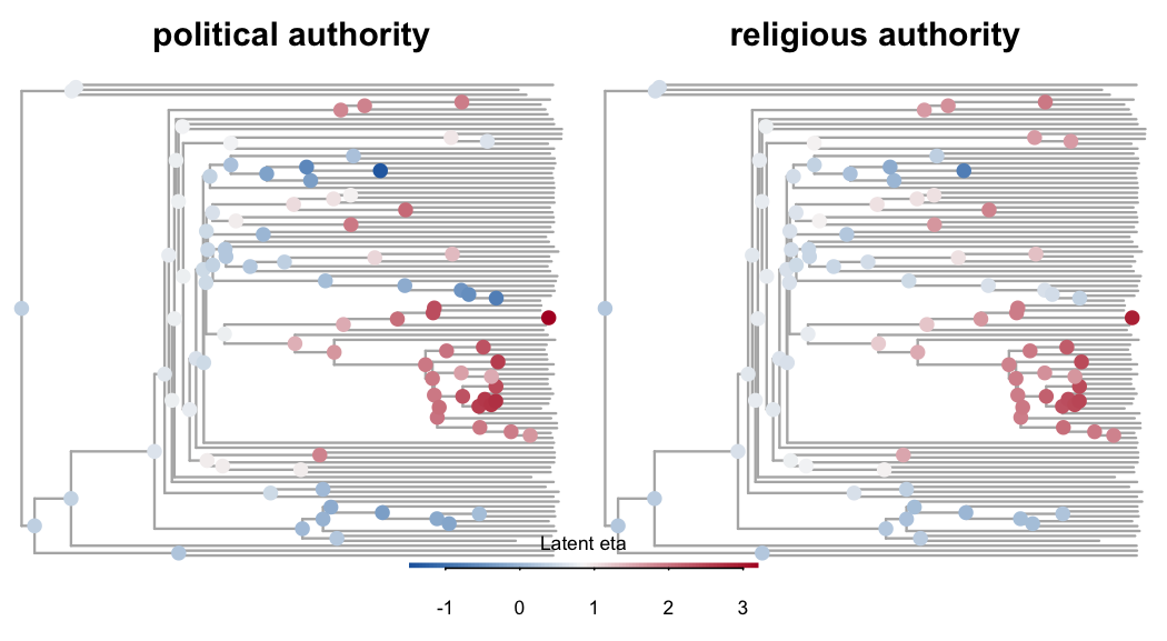
plot of chunk asr-latent-tree
Joint latent-space scatterplot
We can also look at the joint distribution of ancestral states across the two variables. Each point is an internal node, with crosshairs showing the 95% credible interval:
asr_wide <- asr_latent |>
  select(node, variable, estimate, lower, upper) |>
  pivot_wider(
    names_from = variable,
    values_from = c(estimate, lower, upper)
  )

ggplot(asr_wide,
       aes(x = estimate_political_authority,
           y = estimate_religious_authority)) +
  geom_errorbar(
    aes(ymin = lower_religious_authority,
        ymax = upper_religious_authority),
    alpha = 0.2, width = 0
  ) +
  geom_errorbarh(
    aes(xmin = lower_political_authority,
        xmax = upper_political_authority),
    alpha = 0.2, height = 0
  ) +
  geom_point(color = "#B2182B", size = 2) +
  labs(
    x = "Political authority (latent)",
    y = "Religious authority (latent)",
    title = "Ancestral states at internal nodes"
  )
Warning: `geom_errorbarh()` was deprecated in ggplot2 4.0.0.
ℹ Please use the `orientation` argument of `geom_errorbar()` instead.
This warning is displayed once per session.
Call `lifecycle::last_lifecycle_warnings()` to see where this warning was generated.`height` was translated to `width`.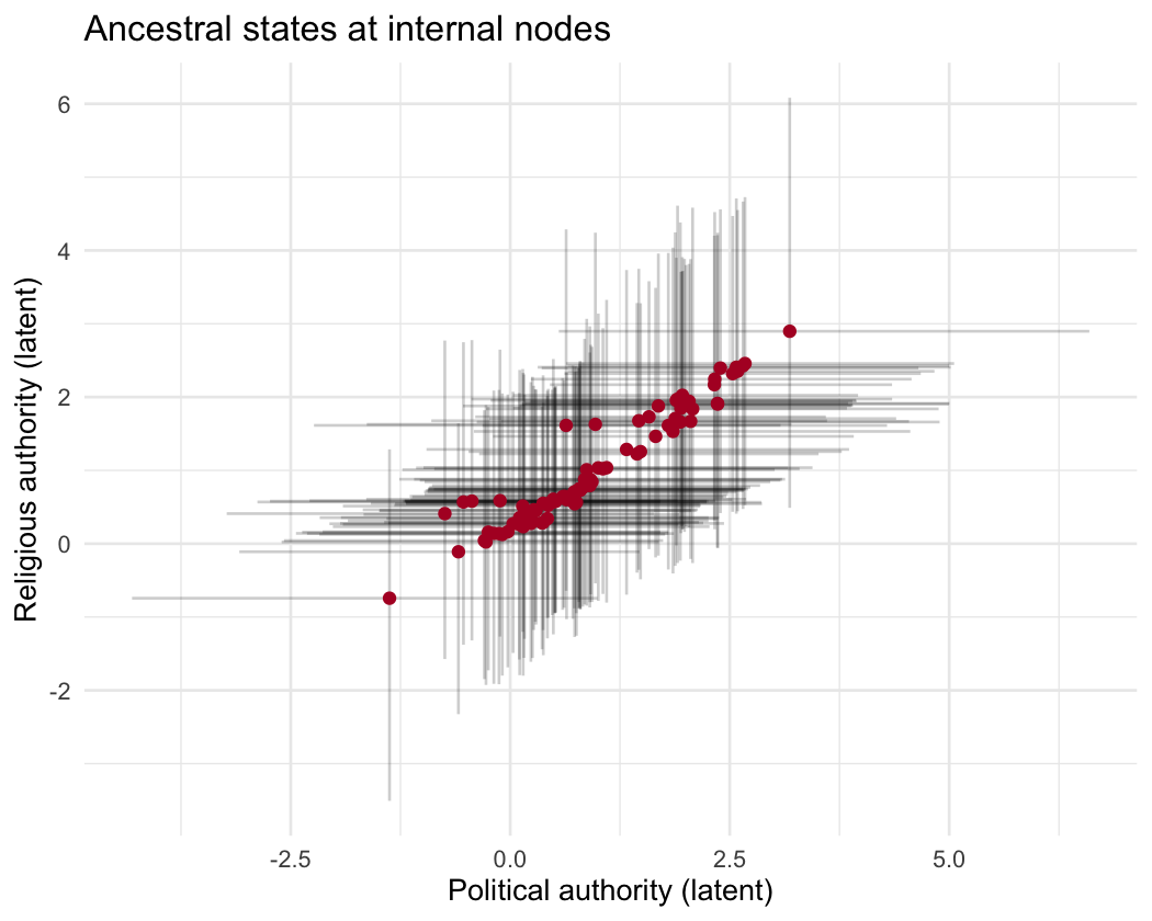
plot of chunk asr-latent-scatter
Ancestral states on the response scale
For ordered-logistic variables, the response scale returns estimated
category probabilities at each node – how likely each level of authority
(absent, sublocal, local, supralocal) was at that ancestral node. Each
ordinal variable expands to one row per category, with
category populated:
asr_resp <- coev_ancestral_states(
  fit, nodes = "all", scale = "response"
)
head(asr_resp, 8)
# A tibble: 8 × 6
node variable category estimate lower upper
<int> <chr> <chr> <dbl> <dbl> <dbl>
1 1 political_authority cat_1 0.0448 0.00200 0.276
2 1 political_authority cat_2 0.0425 0.00220 0.181
3 1 political_authority cat_3 0.349 0.0435 0.600
4 1 political_authority cat_4 0.536 0.115 0.950
5 1 religious_authority cat_1 0.0340 0.00139 0.258
6 1 religious_authority cat_2 0.0275 0.00108 0.154
7 1 religious_authority cat_3 0.335 0.0282 0.593
8 1 religious_authority cat_4 0.584 0.124 0.968The point estimate (estimate) is the posterior median
for all rows, consistent with the latent scale. Because medians do not
distribute over sums, the per-node category estimates need not sum
exactly to 1. The lower and upper columns are
per-category posterior quantiles.
Pie chart tree: response-scale probabilities
This is the most intuitive way to visualize ordinal ancestral states. Each pie chart at an internal node shows the posterior probability of each category (posterior medians, normalized to sum to 1). At the tips, observed values are shown as solid colors (one category with probability 1). If a tip has missing data, the model-estimated probabilities are shown instead.
cat_labels <- c("Absent", "Sublocal", "Local", "Supralocal")
cat_colors <- c("#FFFFB2", "#FECC5C", "#FD8D3C", "#E31A1C")
n_cats <- length(cat_labels)

# pivot ordinal-response long format -> per-node probability matrix
to_pie_mat <- function(df) {
  wide <- df |>
    select(node, category, estimate) |>
    pivot_wider(names_from = category, values_from = estimate) |>
    arrange(node)
  mat <- as.matrix(wide[, paste0("cat_", seq_len(n_cats))])
  mat / rowSums(mat)
}

par(mfrow = c(1, 2), mar = c(1, 0, 3, 0))

for (var in unique(asr_resp$variable)) {
  df_var <- asr_resp |> filter(variable == var)
  plot(tree, show.tip.label = FALSE, edge.width = 1.5,
       edge.color = "grey50", main = gsub("_", " ", var))
  # internal nodes: model-estimated category probabilities
  nodelabels(pie = to_pie_mat(filter(df_var, node > n_tips)),
             piecol = cat_colors, cex = 0.6)
  # tips: observed value (deterministic) when present, otherwise model estimate
  tip_pie <- to_pie_mat(filter(df_var, node <= n_tips))
  obs <- authority$data[[var]][match(tree$tip.label, authority$data$language)]
  observed <- !is.na(obs)
  tip_pie[observed, ] <- 0
  tip_pie[cbind(which(observed), as.integer(obs[observed]))] <- 1
  tiplabels(pie = tip_pie, piecol = cat_colors, cex = 0.4)
}

# shared legend
par(fig = c(0.2, 0.8, 0, 0.12), new = TRUE, mar = rep(0, 4))
plot.new()
legend("center", legend = cat_labels, fill = cat_colors, xpd = NA,
       horiz = TRUE, bty = "n", cex = 0.9, title = "Authority level")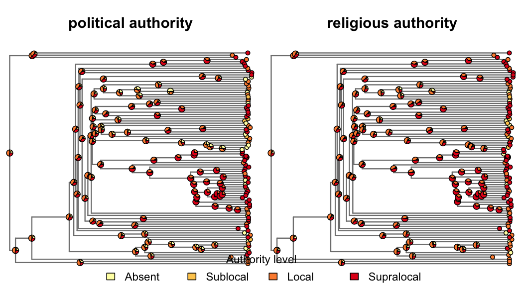
plot of chunk asr-pie-tree
Working with raw posterior draws
Setting summary = FALSE returns the full posterior
array, which is useful for custom summaries or propagating
uncertainty:
asr_draws <- coev_ancestral_states(fit, summary = FALSE)
str(asr_draws, max.level = 1)
List of 4
$ draws : num [1:2000, 1:96, 1:2] 0.447 0.239 1.269 -0.543 0.754 ...
..- attr(*, "dimnames")=List of 3
$ ref_tree :List of 5
..- attr(*, "class")= chr "phylo"
..- attr(*, "order")= chr "cladewise"
..- attr(*, "clade.credibility")= num -24.9
$ node_ids : int [1:96] 98 99 100 101 102 103 104 105 106 107 ...
$ variable_names: chr [1:2] "political_authority" "religious_authority"The draws element is a 3D array with dimensions
[draws, nodes, variables]. Here’s an example: the posterior
density of latent values at the root node for both variables:
root_node_idx <- which(asr_draws$node_ids == n_tips + 1)

root_df <- data.frame(
  political_authority = asr_draws$draws[, root_node_idx, 1],
  religious_authority = asr_draws$draws[, root_node_idx, 2]
) |>
  pivot_longer(everything(), names_to = "variable", values_to = "eta")

ggplot(root_df, aes(x = eta, fill = variable)) +
  geom_density(alpha = 0.5) +
  scale_fill_manual(
    values = c(political_authority = "#2166AC",
               religious_authority = "#B2182B"),
    labels = c("Political", "Religious"),
    name = "Authority"
  ) +
  labs(
    x = "Latent value (eta)",
    y = "Density",
    title = "Posterior distribution at the root node"
  )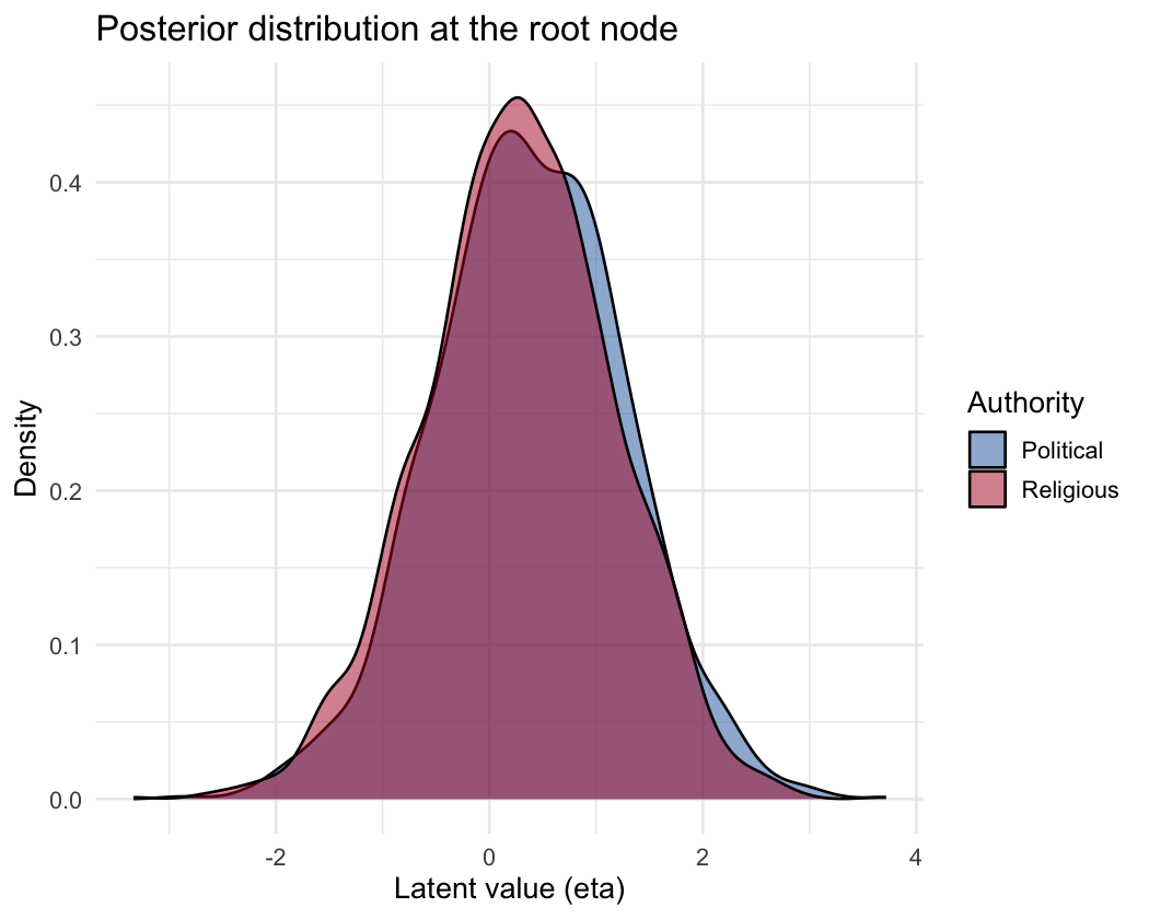
plot of chunk asr-root-density
Identifying nodes on the tree
To query ancestral states for specific nodes, you first need to know
their IDs. Node numbering follows ape’s convention: tips are
1:N_tips and internal nodes are
(N_tips + 1):(2 * N_tips - 1). The ape package provides
everything needed to display and select nodes – for example, plotting
the tree with internal node IDs labelled:
plot(tree, show.tip.label = FALSE, edge.color = "grey70")
nodelabels(cex = 0.5, frame = "circle", bg = "lightblue")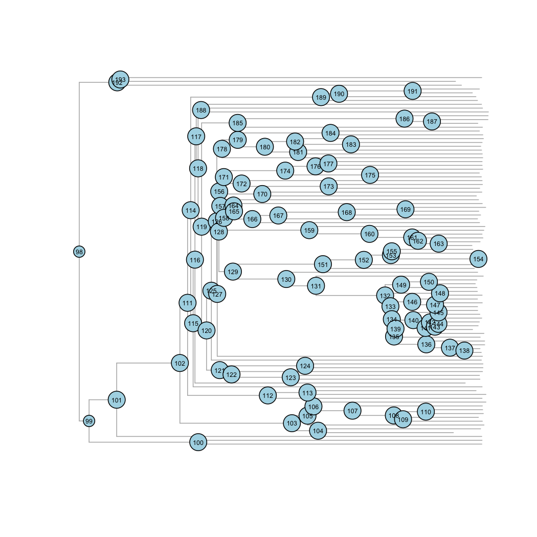
plot of chunk asr-node-labels
In an interactive R session you can instead click directly on the
plotted tree to select nodes with
ape::identify.phylo():
plot(tree, show.tip.label = FALSE)
node <- identify(tree)$nodes
coev_ancestral_states(fit, nodes = node)
Selecting specific nodes and variables
Once you know the node IDs, you can target specific nodes or variables to reduce computation and focus the output:
# only religious authority, at three specific internal nodes
asr_sub <- coev_ancestral_states(
  fit,
  variables = "religious_authority",
  nodes = c(n_tips + 1, n_tips + 2, n_tips + 3)
)
asr_sub
# A tibble: 3 × 5
node variable estimate lower upper
<int> <chr> <dbl> <dbl> <dbl>
1 98 religious_authority 0.300 -1.56 2.20
2 99 religious_authority 0.295 -1.50 2.18
3 100 religious_authority 0.295 -1.71 2.19