Introduction

This vignette provides an introduction to the coevolve package. It briefly describes the class of generalized dynamic phylogenetic models (GDPMs) that the package is designed to fit. It then runs through several working examples to showcase features of the package, including models with different response distributions, missing data, repeated observations, multiPhylo tree objects, and controls for spatial location.

The generalized dynamic phylogenetic model

In the coevolve package, the main function is coev_fit(), which fits a generalized dynamic phylogenetic model to taxa variables given the phylogenetic relationships among taxa. The model allows the user to determine whether evolutionary change in one variable precedes evolutionary change in another variable.

A full description of the model can be found in this pre-print. Briefly, the model represents observed variables as latent variables that are allowed to coevolve along an evolutionary time series. Coevolution unfolds according to a stochastic differential equation similar to an Ornstein-Uhlenbeck process, which contains both “selection” (tendency towards an optimum value) and “drift” (exogenous Gaussian noise) components. Change in the latent variables depend upon all other latent variables in the model and themselves, allowing users to assess the directional influence of one variable on future change in another variable.

Similar dynamic coevolutionary models are offered in programs like BayesTraits (see here). However, these models are limited to a small number of discrete traits. The coevolve package goes beyond these models by allowing the user to estimate coevolutionary effects between any number of variables and a much wider range of response distributions, including continuous, binary, ordinal, and count distributions.

A working example

To show the model in action, we will use data on political and religious authority among 97 Austronesian societies. Political and religious authority are both four-level ordinal variables representing whether each type of authority is absent (not present above the household level), sublocal (incorporating a group larger than the household but smaller than the local community), local (incorporating the local community) and supralocal (incorporating more than one local community). These data were compiled by Sheehan et al. (2023).

library(coevolve)
head(authority$data)
        language political_authority religious_authority
1          Aiwoo            Sublocal            Sublocal
2          Alune          Supralocal          Supralocal
3 AnejomAneityum          Supralocal          Supralocal
4          Anuta               Local               Local
5          Atoni          Supralocal          Supralocal
6          Baree               Local               Local

Each society is on a separate row and is linked to a different Austronesian language. These languages can be represented on a linguistic phylogeny (see authority$phylogeny). We are interested in using this phylogeny to understand how political and religious authority have coevolved over the course of Austronesian cultural evolution.

To fit the generalized dynamic phylogenetic model, we use the coev_fit() function. Internally, this function builds the Stan code, builds a data list, and then compiles and fits the model using the cmdstanr package. Users can run these steps one-by-one using the coev_make_stancode() and coev_make_standata() functions, but for brevity we just use the coev_fit() function.

fit1 <-
  coev_fit(
    data = authority$data,
    variables = list(
      political_authority = "ordered_logistic",
      religious_authority = "ordered_logistic"
    ),
    id = "language",
    tree = authority$phylogeny,
    # set manual prior
    prior = list(A_offdiag = "normal(0, 2)"),
    # return log likelihood
    log_lik = TRUE,
    # additional arguments for cmdstanr
    parallel_chains = 4,
    iter_sampling = 2000,
    iter_warmup = 2000,
    refresh = 0,
    seed = 1
  )
Running MCMC with 4 parallel chains...

Chain 2 finished in 878.0 seconds.
Chain 4 finished in 1213.6 seconds.
Chain 1 finished in 1228.8 seconds.
Chain 3 finished in 1251.5 seconds.

All 4 chains finished successfully.
Mean chain execution time: 1143.0 seconds.
Total execution time: 1252.7 seconds.

The function takes several arguments, including a dataset, a named list of variables that we would like to coevolve in the model (along with their associated response distributions), the column in the dataset that links to the phylogeny tip labels, and a phylogeny of class phylo. The function sets priors for the parameters by default, but it is possible for the user to manually set these priors. The user can also pass additional arguments to cmdstanr’s sample() method which runs under the hood.

Once the model has fitted, we can print a summary of the parameters.

summary(fit1)
Variables: political_authority = ordered_logistic 
           religious_authority = ordered_logistic 
     Data: authority$data (Number of observations: 97)
Phylogeny: authority$phylogeny (Number of trees: 1)
    Draws: 4 chains, each with iter = 2000; warmup = 2000; thin = 1
           total post-warmup draws = 8000

Autoregressive selection effects:
                    Estimate Est.Error  2.5% 97.5% Rhat Bulk_ESS Tail_ESS
political_authority    -0.67      0.52 -1.97 -0.03 1.00     5036     4459
religious_authority    -0.78      0.57 -2.13 -0.03 1.00     5461     3926

Cross selection effects:
                                          Estimate Est.Error  2.5% 97.5% Rhat Bulk_ESS Tail_ESS
political_authority ⟶ religious_authority     2.28      0.99  0.34  4.26 1.00     3310     3706
religious_authority ⟶ political_authority     1.81      1.11 -0.36  4.08 1.00     2068     3963

Drift parameters:
                                             Estimate Est.Error  2.5% 97.5% Rhat Bulk_ESS Tail_ESS
sd(political_authority)                          1.93      0.82  0.25  3.45 1.00     1446     1572
sd(religious_authority)                          1.27      0.79  0.06  2.91 1.00     1478     3513
cor(political_authority,religious_authority)     0.26      0.31 -0.42  0.77 1.00     5593     6287

Continuous time intercept parameters:
                    Estimate Est.Error  2.5% 97.5% Rhat Bulk_ESS Tail_ESS
political_authority     0.21      0.94 -1.65  2.01 1.00     8762     5444
religious_authority     0.21      0.94 -1.66  2.06 1.00     9553     5646

Ordinal cutpoint parameters:
                       Estimate Est.Error  2.5% 97.5% Rhat Bulk_ESS Tail_ESS
political_authority[1]    -1.29      0.89 -3.03  0.51 1.00     5964     5452
political_authority[2]    -0.55      0.87 -2.22  1.20 1.00     6278     5920
political_authority[3]     1.65      0.91 -0.08  3.49 1.00     6729     6160
religious_authority[1]    -1.51      0.92 -3.30  0.29 1.00     6792     5557
religious_authority[2]    -0.82      0.90 -2.58  0.97 1.00     7241     6064
religious_authority[3]     1.60      0.93 -0.15  3.49 1.00     6983     6370
Warning: There were 18 divergent transitions after warmup.
http://mc-stan.org/misc/warnings.html#divergent-transitions-after-warmup

We can see a printed summary of the model parameters, including the autoregressive effects (i.e., the effects of variables on themselves in the future), the cross effects (i.e., the effects of variables on the other variables in the future), the amount of drift, correlated drift, the continuous time intercepts for the stochastic differential equation, and the ordinal cutpoints for both variables.

While the summary output is useful, it is difficult to interpret the parameters directly to make inferences about coevolutionary patterns. An alternative approach is to directly “intervene” in the system. By doing this, we can better understand how increases or decreases in a variable change the equilibrium trait values of other variables in the system. For example, we can hold one variable at its average value and then increase it by a standardised amount to see how the equilibrium value for the other trait changes.

The function coev_calculate_delta_theta() allows the user to calculate \(\Delta\theta_{z}\), which is defined as the change in the equilibrium trait value for one variable which results from a median absolute deviation increase in another variable. This function returns a posterior distribution. We can easily visualise the posterior distributions for all cross effects at once using the function coev_plot_delta_theta().

plot of chunk authority-delta-theta

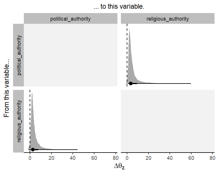
This plot shows the posterior distribution, the posterior median, and the 66% and 95% credible intervals for \(\Delta\theta_{z}\). We can conclude that political and religious authority both influence each other in their evolution. A one median absolute deviation increase in political authority results in an increase in the equilibrium trait value for religious authority, and vice versa. In other words, these two variables coevolve reciprocally over time.

There are several ways to visualise this runaway coevolutionary process: (1) a flow field of evolutionary change, (2) a selection gradient plot, and (3) a time series simulation of evolutionary dynamics. In order to make these various plots more understandable, it is useful to first plot where the different taxa are situated in latent trait space. We can do this using the coev_plot_trait_values() function, which produces a pairs plot of estimated trait values for all the variables in the model (along with associated posterior uncertainty on the diagonal).

coev_plot_trait_values(fit1, xlim = c(-5, 7), ylim = c(-5, 7))

plot of chunk authority-trait-values

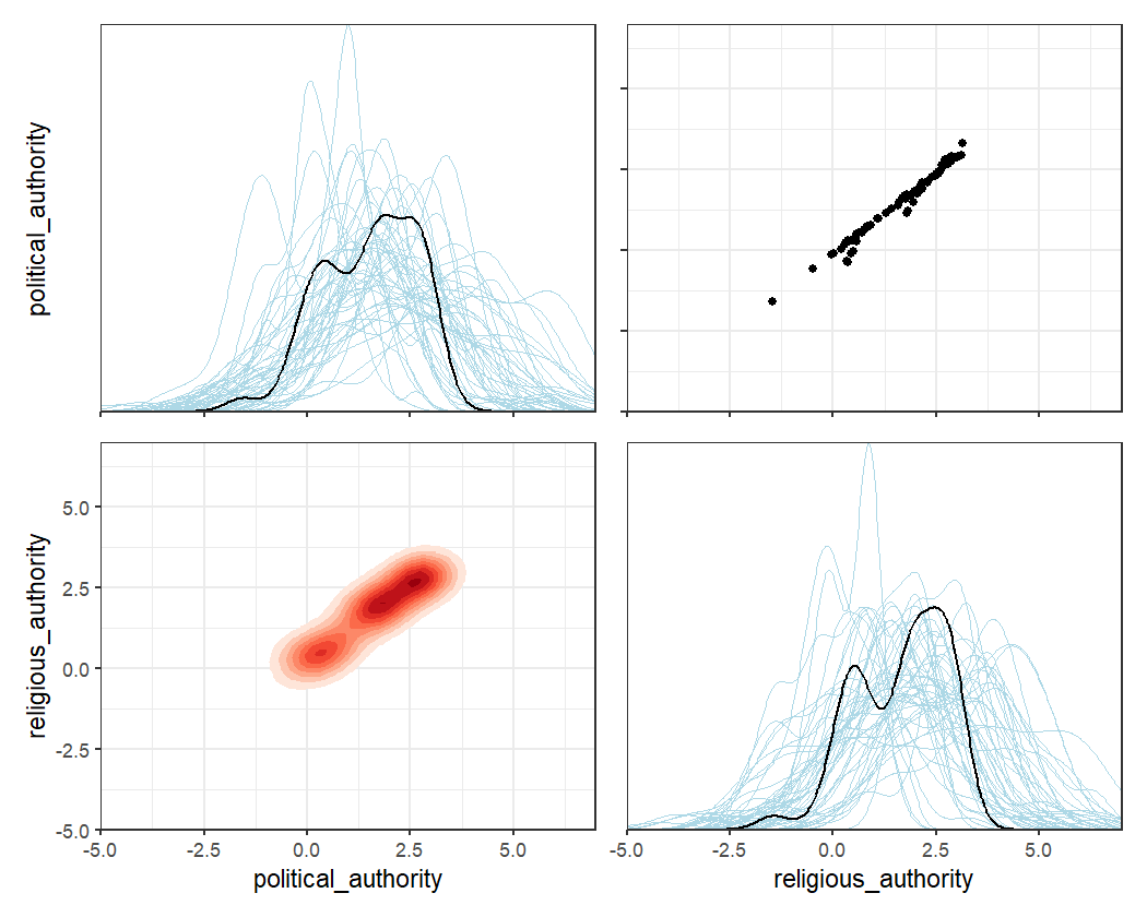
Now that we have a good sense of the trait space, we can plot a flow field of evolutionary change. The coev_plot_flowfield() function plots the strength and direction of evolutionary change at different locations in trait space.

coev_plot_flowfield(
  object = fit1,
  var1 = "political_authority",
  var2 = "religious_authority",
  limits = c(-5, 5)
  )

plot of chunk authority-flowfield

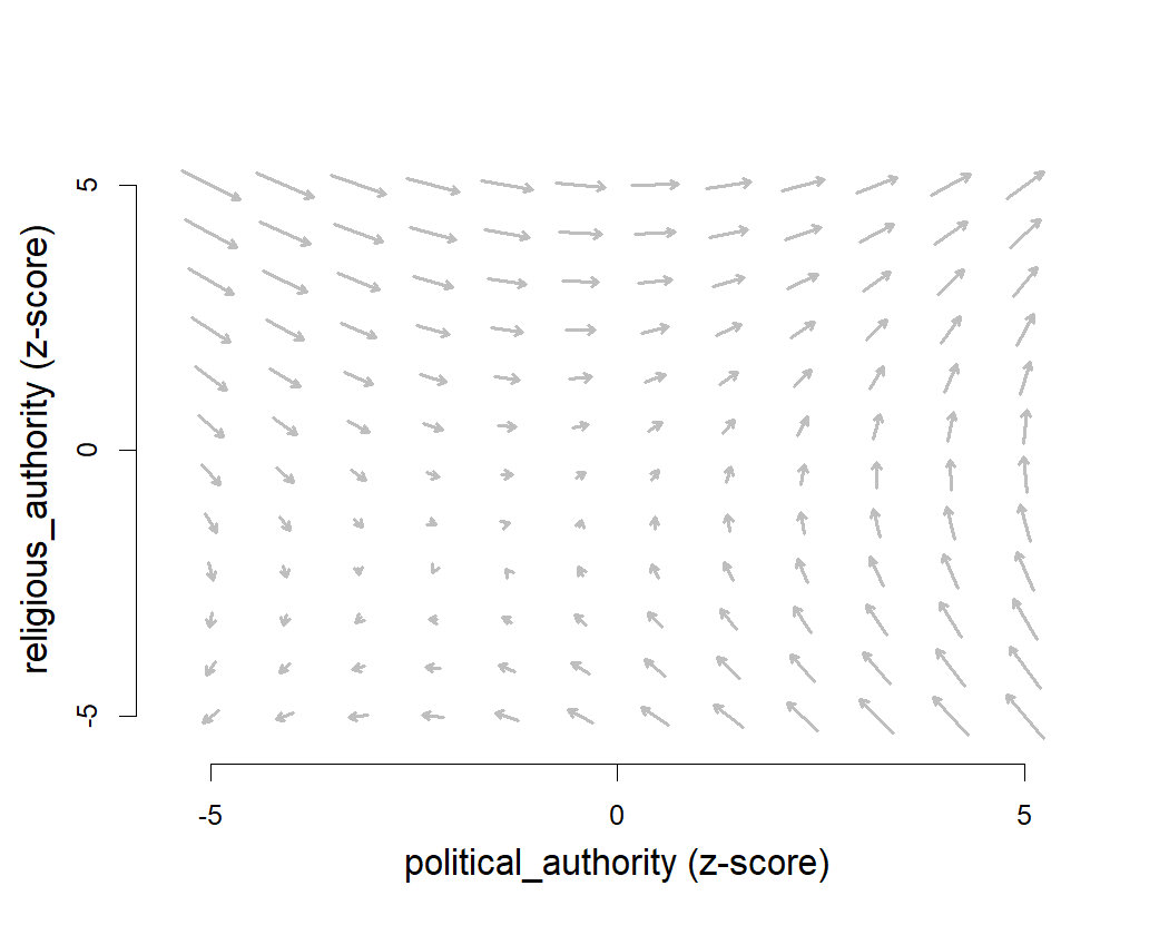
The arrows in this plot tend to point towards the upper right-hand corner, suggesting that political and religious authority evolve towards higher levels in a runaway coevolutionary process.

We can also visualise the coevolutionary dynamics with a selection gradient plot. The function coev_plot_selection_gradient() produces a heatmap which shows how selection acts on both variables at different locations in trait space, with green indicating positive selection and red indicating negative selection.

coev_plot_selection_gradient(
  object = fit1,
  var1 = "political_authority",
  var2 = "religious_authority",
  limits = c(-5, 5)
)

plot of chunk authority-selection-gradient

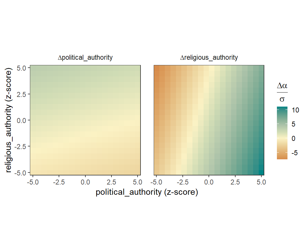
We can see from this plot that as each variable increases, the selection on the other variable increases.

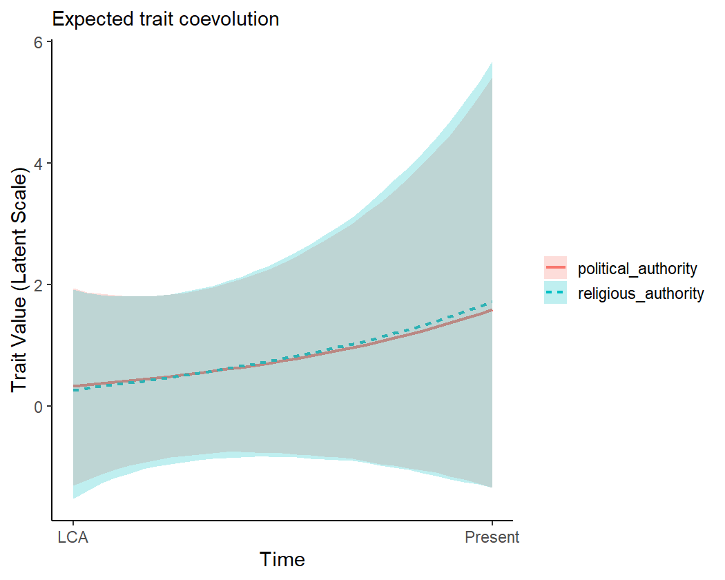
Finally, we can “replay the past” by simulating these coevolutionary dynamics over a time series. By default, the coev_plot_pred_series() function uses the model-implied ancestral states at the root of the phylogeny as starting points, and allows the variables to coevolve over time. Shaded areas represent 95% credible intervals for the predictions.

plot of chunk authority-pred-series-1

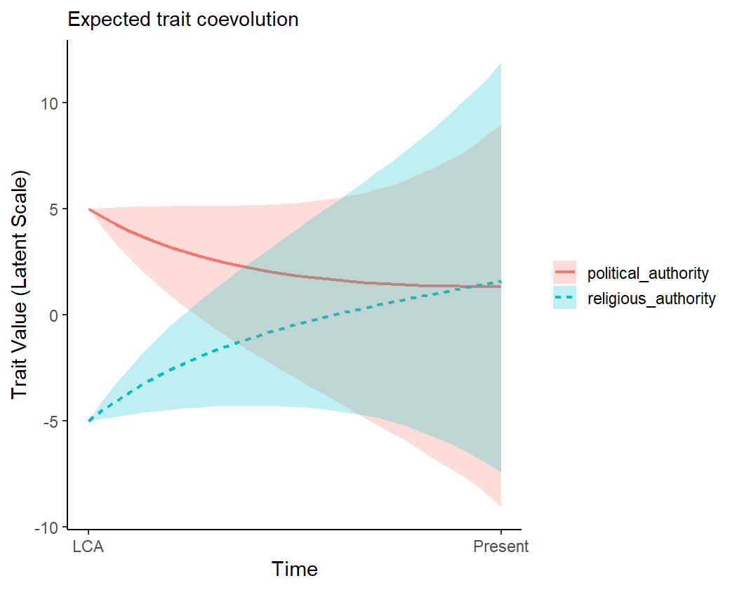
It is also possible to initialise the variables at different starting points, to see the implied coevolutionary dynamics. For example, we can imagine a case where the ancestral society had high levels of political authority but low levels of religious authority.

coev_plot_pred_series(
  object = fit1,
  eta_anc = list(
    political_authority = 5,
    religious_authority = -5
  )
)

plot of chunk authority-pred-series-2

Available response distributions

In the above example, both variables were ordinal. As such, we declared both of them to follow the “ordered_logistic” response distribution. But the coevolve package supports several more response distributions.

Response distribution Data type Link function
bernoulli_logit Binary Logit
ordered_logistic Ordinal Logit
poisson_softplus Count Softplus
negative_binomial_softplus Count Softplus
normal Continuous real -
gamma_log Positive real Log

Different variables need not follow the same response distribution. This can be useful when users would like to assess the coevolution between variables of different types.

Handling missing data

Often in comparative datasets, data will be missing for some taxa. Rather than remove cases if they have any missing data, the coev_fit() function will automatically impute any missing values in the model, using all available information.

We show this by modelling the coevolutionary relationships between brain weight and group size across 21 primate species from the Lemuriformes clade. Data on primate species were compiled by DeCasien et al. (2017). There are data for 143 primate species in total, but we focus on one clade to keep the example small and simple.

# filter dataset to Lemuriformes only
primates_data <- primates$data[primates$data$clade == "Lemuriformes",]

# prune phylogeny to Lemuriformes only
library(ape)
primates_phylogeny <- keep.tip(primates$phylogeny, primates_data$species)

# view data
head(primates_data[, c("species", "brain_weight", "group_size")])
                        species brain_weight group_size
13                Avahi_laniger    10.251355   2.666667
14           Avahi_occidentalis     8.236200         NA
44           Cheirogaleus_major     6.119797   5.500000
45          Cheirogaleus_medius     2.912291   2.000000
54 Daubentonia_madagascariensis    46.344725   1.750000
56            Eulemur_coronatus    21.394398   6.950000

Both variables are positive reals, so we use the “gamma_log” distribution. While there are no missing data for the brain weight variable, some data are missing for the group size variable.

fit2 <-
  coev_fit(
    data = primates_data,
    variables = list(
      brain_weight = "gamma_log",
      group_size = "gamma_log"
    ),
    id = "species",
    tree = primates_phylogeny,
    # additional arguments for cmdstanr
    parallel_chains = 4,
    iter_sampling = 2000,
    iter_warmup = 2000,
    refresh = 0,
    seed = 1
  )
Running MCMC with 4 parallel chains...

Chain 1 finished in 459.8 seconds.
Chain 3 finished in 477.3 seconds.
Chain 2 finished in 607.5 seconds.
Chain 4 finished in 634.7 seconds.

All 4 chains finished successfully.
Mean chain execution time: 544.8 seconds.
Total execution time: 634.8 seconds.
summary(fit2)
Variables: brain_weight = gamma_log 
           group_size = gamma_log 
     Data: primates_data (Number of observations: 21)
Phylogeny: primates_phylogeny (Number of trees: 1)
    Draws: 4 chains, each with iter = 2000; warmup = 2000; thin = 1
           total post-warmup draws = 8000

Autoregressive selection effects:
             Estimate Est.Error  2.5% 97.5% Rhat Bulk_ESS Tail_ESS
brain_weight    -0.42      0.35 -1.34 -0.01 1.00     5998     3875
group_size      -0.77      0.54 -2.01 -0.04 1.00     6044     3424

Cross selection effects:
                          Estimate Est.Error  2.5% 97.5% Rhat Bulk_ESS Tail_ESS
brain_weight ⟶ group_size     0.46      0.72 -1.12  1.76 1.00     2799     2861
group_size ⟶ brain_weight     0.62      0.94 -1.29  2.41 1.00     3113     3754

Drift parameters:
                             Estimate Est.Error  2.5% 97.5% Rhat Bulk_ESS Tail_ESS
sd(brain_weight)                 1.07      0.22  0.67  1.56 1.00     2112     2198
sd(group_size)                   0.69      0.44  0.04  1.66 1.01      784     1713
cor(brain_weight,group_size)     0.06      0.30 -0.53  0.62 1.00     7637     5552

Continuous time intercept parameters:
             Estimate Est.Error  2.5% 97.5% Rhat Bulk_ESS Tail_ESS
brain_weight    -0.25      0.85 -1.88  1.41 1.00     5417     5515
group_size      -0.87      0.76 -2.32  0.66 1.00     5891     5285

Shape parameters:
             Estimate Est.Error 2.5%  97.5% Rhat Bulk_ESS Tail_ESS
brain_weight    57.29     60.33 4.83 223.56 1.01      573     1593
group_size       5.99     12.12 1.43  28.40 1.01      826      784
Warning: There were 91 divergent transitions after warmup.
http://mc-stan.org/misc/warnings.html#divergent-transitions-after-warmup

Notice that the number of observations is still 21 in the summary output, informing us that all observations were retained and any missing data were imputed.

If we wanted instead to remove any taxa with missing data, we could set complete_cases = TRUE when fitting the model.

Repeated observations

Another common feature of comparative datasets is repeated observations. In the previous examples, we had only one observation per taxon. But often there will be more than one observation for each taxon, such as when we have observed multiple individuals of the same species. In these cases, it can be useful to include all of these observations in the model and estimate the residual variation that is not due to the coevolutionary process.

We show this using an example dataset from de Villemereuil & Nakagawa (2014). Suppose we have measured two continuous variables (\(x\) and \(y\)) for 20 species, with five observations for each species.

head(repeated$data)
  species         x         y
1    sp_1 11.223724 107.41919
2    sp_1  9.805934 109.16403
3    sp_1 10.308423  91.88672
4    sp_1  8.355349 121.54341
5    sp_1 11.854510 105.31638
6    sp_2  4.314015  64.99859

We can fit the dynamic coevolutionary model to this dataset.

fit3 <-
  coev_fit(
    data = repeated$data,
    variables = list(
      x = "normal",
      y = "normal"
    ),
    id = "species",
    tree = repeated$phylogeny,
    # additional arguments for cmdstanr
    parallel_chains = 4,
    iter_warmup = 2000,
    iter_sampling = 2000,
    refresh = 0,
    seed = 1
  )
Running MCMC with 4 parallel chains...

Chain 2 finished in 605.4 seconds.
Chain 4 finished in 624.9 seconds.
Chain 3 finished in 851.5 seconds.
Chain 1 finished in 852.4 seconds.

All 4 chains finished successfully.
Mean chain execution time: 733.5 seconds.
Total execution time: 852.4 seconds.
summary(fit3)
Variables: x = normal 
           y = normal 
     Data: repeated$data (Number of observations: 100)
Phylogeny: repeated$phylogeny (Number of trees: 1)
    Draws: 4 chains, each with iter = 2000; warmup = 2000; thin = 1
           total post-warmup draws = 8000

Autoregressive selection effects:
  Estimate Est.Error  2.5% 97.5% Rhat Bulk_ESS Tail_ESS
x    -1.57      0.77 -3.18 -0.20 1.00     3920     2089
y    -1.32      0.71 -2.78 -0.12 1.00     4906     3238

Cross selection effects:
      Estimate Est.Error  2.5% 97.5% Rhat Bulk_ESS Tail_ESS
x ⟶ y     0.42      0.85 -1.25  2.07 1.00     6608     5754
y ⟶ x     0.03      0.87 -1.71  1.73 1.00     6875     5415

Drift parameters:
         Estimate Est.Error 2.5% 97.5% Rhat Bulk_ESS Tail_ESS
sd(x)        2.94      0.32 2.37  3.63 1.00     4183     5327
sd(y)        2.58      0.29 2.05  3.20 1.00     4666     5667
cor(x,y)     0.88      0.06 0.72  0.96 1.00     3234     4999

Continuous time intercept parameters:
  Estimate Est.Error  2.5% 97.5% Rhat Bulk_ESS Tail_ESS
x    -0.03      0.79 -1.59  1.51 1.00     6792     6144
y     0.06      0.78 -1.51  1.58 1.00     7337     5761

Residual parameters:
         Estimate Est.Error  2.5% 97.5% Rhat Bulk_ESS Tail_ESS
sd(x)        0.28      0.02  0.23  0.33 1.00     8310     5374
sd(y)        0.29      0.02  0.25  0.34 1.00     8427     5323
cor(x,y)    -0.18      0.11 -0.38  0.03 1.00     7568     5759
Warning: There were 36 divergent transitions after warmup.
http://mc-stan.org/misc/warnings.html#divergent-transitions-after-warmup

In the model output, we can see that coev_fit() has detected the presence of repeated observations and has consequently modelled residual standard deviation and residual correlation parameters for \(x\) and \(y\).

Using multiPhylo tree objects

Often, we would like to average our analysis over a posterior set of phylogenetic trees, rather than use a single tree. This can be a useful way to account for phylogenetic uncertainty in our inferences.

To deal with phylogenetic uncertainty, the coev_fit() function allows the user to declare multiPhylo objects in the tree argument. So long as all trees in the multiPhylo object have the same number of taxa with the same tip labels, the Stan code will average over all the trees within the same model.

To keep the computation time short, we imagine a simple case where we have a multiPhylo object with two identical Austronesian language phylogenies. While the results should be the same in this case as there is no phylogenetic uncertainty, users should expect differing results when using sets of different trees.

authority_multiphylo <- c(
  authority$phylogeny,
  authority$phylogeny
)

authority_multiphylo
2 phylogenetic trees
fit4 <-
  coev_fit(
    data = authority$data,
    variables = list(
      political_authority = "ordered_logistic",
      religious_authority = "ordered_logistic"
    ),
    id = "language",
    # use multiPhylo tree object
    tree = authority_multiphylo,
    # set manual prior
    prior = list(A_offdiag = "normal(0, 2)"),
    # additional arguments for cmdstanr
    parallel_chains = 4,
    iter_sampling = 2000,
    iter_warmup = 2000,
    refresh = 0,
    seed = 1
  )
Running MCMC with 4 parallel chains...

Chain 4 finished in 1598.6 seconds.
Chain 3 finished in 1625.2 seconds.
Chain 2 finished in 1633.5 seconds.
Chain 1 finished in 2088.5 seconds.

All 4 chains finished successfully.
Mean chain execution time: 1736.5 seconds.
Total execution time: 2088.7 seconds.
summary(fit4)
Variables: political_authority = ordered_logistic 
           religious_authority = ordered_logistic 
     Data: authority$data (Number of observations: 97)
Phylogeny: authority_multiphylo (Number of trees: 2)
    Draws: 4 chains, each with iter = 2000; warmup = 2000; thin = 1
           total post-warmup draws = 8000

Autoregressive selection effects:
                    Estimate Est.Error  2.5% 97.5% Rhat Bulk_ESS Tail_ESS
political_authority    -0.64      0.52 -1.95 -0.02 1.00     5950     3489
religious_authority    -0.70      0.55 -2.07 -0.03 1.00     6287     4187

Cross selection effects:
                                          Estimate Est.Error 2.5% 97.5% Rhat Bulk_ESS Tail_ESS
political_authority ⟶ religious_authority     2.05      1.03 0.37  4.34 1.00     2690     5116
religious_authority ⟶ political_authority     2.12      1.08 0.26  4.47 1.00     2419     3669

Drift parameters:
                                             Estimate Est.Error  2.5% 97.5% Rhat Bulk_ESS Tail_ESS
sd(political_authority)                          1.11      0.83  0.04  2.94 1.00      910     2354
sd(religious_authority)                          0.88      0.68  0.03  2.50 1.00     1456     2887
cor(political_authority,religious_authority)     0.05      0.33 -0.60  0.66 1.00     4522     5683

Continuous time intercept parameters:
                    Estimate Est.Error  2.5% 97.5% Rhat Bulk_ESS Tail_ESS
political_authority     0.34      0.91 -1.43  2.11 1.00     9445     6549
religious_authority     0.42      0.92 -1.40  2.18 1.00    10164     5564

Ordinal cutpoint parameters:
                       Estimate Est.Error  2.5% 97.5% Rhat Bulk_ESS Tail_ESS
political_authority[1]    -1.55      0.90 -3.36  0.15 1.00     6041     5141
political_authority[2]    -0.81      0.88 -2.59  0.85 1.00     6578     5453
political_authority[3]     1.92      0.95  0.11  3.83 1.00     7628     5767
religious_authority[1]    -1.83      0.88 -3.62 -0.13 1.00     6347     5593
religious_authority[2]    -1.15      0.85 -2.87  0.52 1.00     7035     5596
religious_authority[3]     1.67      0.93 -0.06  3.61 1.00     4677     4682
Warning: There were 18 divergent transitions after warmup.
http://mc-stan.org/misc/warnings.html#divergent-transitions-after-warmup

The summary output correctly shows that we averaged over two trees. Note that with more trees, users should expect the computation time for these models to increase.

Controlling for spatial location

If we have data on the spatial location of taxa, sometimes it is useful to control for this spatial location to ensure that our model is capturing deep ancestral relationships rather than more recent diffusion among neighbours. For example, when studying the coevolution of political and religious authority in Austronesian societies, we would like to ensure that our results are due to coevolution over deep cultural time rather than more recent borrowing among societies with close geographic proximity.

The dist_mat argument in the coev_fit() function allows us to easily control for spatial proximity. This argument takes a distance matrix between all taxa in the phylogeny. If the distance matrix is specified by the user, the function includes in the Stan code a separate Gaussian Process over spatial location for each variable in the model.

Here is the geographic distance matrix (measured in metres) for the first five Austronesian societies:

authority$distance_matrix[1:5, 1:5]
                   Aiwoo     Alune AnejomAneityum     Anuta     Atoni
Aiwoo                0.0 4250625.9      1158010.2  408692.9 4602028.5
Alune          4250625.9       0.0      4863176.7 4649868.1  865094.2
AnejomAneityum 1158010.2 4863176.7            0.0  951671.2 5013641.1
Anuta           408692.9 4649868.1       951671.2       0.0 4977783.9
Atoni          4602028.5  865094.2      5013641.1 4977783.9       0.0

We can include this distance matrix in the model. The matrix is scaled to vary between 0 and 1 under the hood to improve model sampling.

fit5 <-
  coev_fit(
    data = authority$data,
    variables = list(
      political_authority = "ordered_logistic",
      religious_authority = "ordered_logistic"
    ),
    id = "language",
    tree = authority$phylogeny,
    # declare distance matrix and covariance kernel
    dist_mat = authority$distance_matrix,
    dist_cov = "exp_quad",
    # set manual prior
    prior = list(A_offdiag = "normal(0, 2)"),
    # return log likelihood
    log_lik = TRUE,
    # additional arguments for cmdstanr
    parallel_chains = 4,
    iter_sampling = 2000,
    iter_warmup = 2000,
    refresh = 0,
    seed = 1
  )
Running MCMC with 4 parallel chains...
Chain 3 finished in 1566.6 seconds.
Chain 1 finished in 1660.9 seconds.
Chain 4 finished in 2080.0 seconds.
Chain 2 finished in 2086.5 seconds.

All 4 chains finished successfully.
Mean chain execution time: 1848.5 seconds.
Total execution time: 2086.7 seconds.
summary(fit5)
Variables: political_authority = ordered_logistic 
           religious_authority = ordered_logistic 
     Data: authority$data (Number of observations: 97)
Phylogeny: authority$phylogeny (Number of trees: 1)
    Draws: 4 chains, each with iter = 2000; warmup = 2000; thin = 1
           total post-warmup draws = 8000

Autoregressive selection effects:
                    Estimate Est.Error  2.5% 97.5% Rhat Bulk_ESS Tail_ESS
political_authority    -0.69      0.54 -1.99 -0.03 1.00     5230     3961
religious_authority    -0.77      0.58 -2.15 -0.03 1.00     5743     3919

Cross selection effects:
                                          Estimate Est.Error  2.5% 97.5% Rhat Bulk_ESS Tail_ESS
political_authority ⟶ religious_authority     2.02      1.19 -0.45  4.34 1.00     2142     2494
religious_authority ⟶ political_authority     1.65      1.23 -0.81  4.06 1.00     2656     3526

Drift parameters:
                                             Estimate Est.Error  2.5% 97.5% Rhat Bulk_ESS Tail_ESS
sd(political_authority)                          1.52      0.80  0.11  3.11 1.00     1181     2182
sd(religious_authority)                          1.02      0.69  0.05  2.54 1.00     1427     2927
cor(political_authority,religious_authority)     0.16      0.33 -0.51  0.74 1.00     5589     5523

Continuous time intercept parameters:
                    Estimate Est.Error  2.5% 97.5% Rhat Bulk_ESS Tail_ESS
political_authority     0.32      0.94 -1.52  2.16 1.00     8469     5212
religious_authority     0.30      0.97 -1.60  2.17 1.00     7767     5844

Ordinal cutpoint parameters:
                       Estimate Est.Error  2.5% 97.5% Rhat Bulk_ESS Tail_ESS
political_authority[1]    -1.49      0.98 -3.41  0.44 1.00     5038     5486
political_authority[2]    -0.77      0.96 -2.64  1.16 1.00     4991     5665
political_authority[3]     1.38      1.01 -0.58  3.42 1.00     4106     5215
religious_authority[1]    -1.62      1.01 -3.58  0.38 1.00     6003     5297
religious_authority[2]    -0.96      1.00 -2.84  1.01 1.00     6071     5604
religious_authority[3]     1.46      1.04 -0.52  3.56 1.00     5740     5616

Gaussian Process parameters for distances:
                          Estimate Est.Error 2.5% 97.5% Rhat Bulk_ESS Tail_ESS
rho(political_authority)      0.05      0.09 0.00  0.33 1.00     1110     2047
rho(religious_authority)      0.06      0.11 0.00  0.39 1.00      626     2322
sdgp(political_authority)     1.82      1.21 0.16  4.73 1.00     1871     1720
sdgp(religious_authority)     2.12      1.40 0.16  5.34 1.01     1185     2182
Warning: There were 630 divergent transitions after warmup.
http://mc-stan.org/misc/warnings.html#divergent-transitions-after-warmup

The summary output shows that the model has estimated the parameters for two Gaussian Process functions over geographic locations, one for each variable.

Model comparison

When we set log_lik = TRUE, the underlying Stan code for these models returns a log likelihood vector for all observations. With this, it is possible to compare different models using methods like approximate leave-one-out cross-validation. For example, we can use the loo_compare() function from the loo package to see whether adding the distance matrix in the authority example improved our out-of-sample predictive accuracy.

library(loo)
loo_compare(
  list(
    fit1 = fit1$fit$loo(), # authority model without distance matrix
    fit5 = fit5$fit$loo()  # authority model with distance matrix
  )
)
     elpd_diff se_diff
fit5  0.0       0.0   
fit1 -1.9       2.8   

This model comparison suggests that adding spatial location to the model did not improve out-of-sample predictive accuracy.

This model comparison approach may also be useful for comparing models with different cross selection effects constrained to zero (see the effects_mat argument in the coev_fit() function). The user can then test whether “turning on” a particular cross selection effect improves model fit. However, currently it is not possible to compare models that include different coevolving variables, as the datasets and resulting log likelihood vectors vary between models.

Conclusion

We hope that this package is a useful addition to the phylogenetic comparative methods toolkit. If you have any questions about the package, please feel free to email Scott Claessens () or Erik Ringen () or raise an issue over on GitHub: https://github.com/ScottClaessens/coevolve/issues

References

DeCasien, A. R., Williams, S. A., & Higham, J. P. (2017). Primate brain size is predicted by diet but not sociality. Nature Ecology & Evolution, 1(5), 0112.

de Villemereuil P. & Nakagawa, S. (2014). General quantitative genetic methods for comparative biology. In L. Garamszegi (Ed.), Modern phylogenetic comparative methods and their application in evolutionary biology: concepts and practice (pp. 287-303). Springer, New York.

Sheehan, O., Watts, J., Gray, R. D., Bulbulia, J., Claessens, S., Ringen, E. J., & Atkinson, Q. D. (2023). Coevolution of religious and political authority in Austronesian societies. Nature Human Behaviour, 7(1), 38-45.